Linear regression on the weather data

Examples

We predict the wind peak in Luzern five hours ahead.

One predictor

import numpy as np
import pandas as pd
import matplotlib.pyplot as plt
from matplotlib.colors import LogNorm
from sklearn.linear_model import LinearRegression
from sklearn.metrics import mean_squared_error

weather = pd.read_csv("https://go.epfl.ch/bio322-weather2015-2018.csv")

train = pd.DataFrame({
    "LUZ_pressure": weather["LUZ_pressure"][:-5].values,
    "wind_peak_in5h": weather["LUZ_wind_peak"][5:].values,
})
train.head()

	LUZ_pressure	wind_peak_in5h
0	980.0	15.5
1	979.9	13.0
2	980.0	12.6
3	980.2	15.5
4	980.5	17.3

X = train[["LUZ_pressure"]].values
y = train["wind_peak_in5h"].values

m1 = LinearRegression().fit(X, y)
print("intercept:", round(float(m1.intercept_), 2))
print("slope:    ", round(float(m1.coef_[0]), 4))

intercept: 346.4
slope:     -0.3447

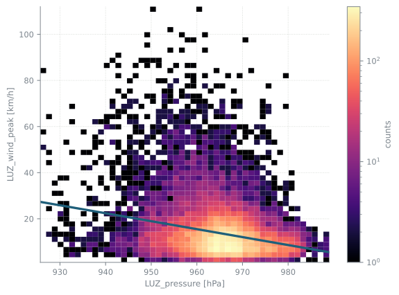
The slope is negative. Lower pressure now means more wind in five hours.

m1.predict(np.array([[930.], [960.], [990.]])).round(2)

array([25.84, 15.5 ,  5.16])

fig, ax = plt.subplots()
h = ax.hist2d(X[:, 0], y, bins=(50, 50), norm=LogNorm(), cmap="magma")
fig.colorbar(h[3], ax=ax, label="counts")
ax.plot(X[:, 0], m1.predict(X), lw=2.5, color="#1f5f7a")
ax.set(xlabel="LUZ_pressure [hPa]", ylabel="LUZ_wind_peak [km/h]")
plt.show()

Figure 10.1: The fitted line on top of the data.

Training and test error

We report the root mean squared error, because it is in the same units as the response.

weather_test = pd.read_csv("https://go.epfl.ch/bio322-weather2019-2020.csv")
test = pd.DataFrame({
    "LUZ_pressure": weather_test["LUZ_pressure"][:-5].values,
    "wind_peak_in5h": weather_test["LUZ_wind_peak"][5:].values,
})

rmse_train = mean_squared_error(y, m1.predict(X)) ** 0.5
rmse_test = mean_squared_error(test["wind_peak_in5h"],
                               m1.predict(test[["LUZ_pressure"]])) ** 0.5
print(f"training RMSE: {rmse_train:.3f}")
print(f"test RMSE:     {rmse_test:.3f}")

training RMSE: 10.006
test RMSE:     11.518

The test set here is a different set of years, so it is a genuinely fresh sample.

Multiple predictors

With \(p\) predictors the model is

\[ \hat y = \beta_0 + \beta_1 x_1 + \cdots + \beta_p x_p. \]

With two predictors the model is a plane. On the left the twenty training points in blue, the plane in green, and the residuals in red: the vertical distances between the plane and the data, which are what least squares makes small. Drag that panel to turn the box, or focus it and use the arrow keys. The loss now depends on three parameters, which is one too many to draw, so on the right are two slices through it: the loss over \(\beta_0\) and \(\beta_1\) with \(\beta_2\) held at the value the slider is on, and the loss over \(\beta_0\) and \(\beta_2\) with \(\beta_1\) held. Moving the third slider does not change the shape of a slice, only where its centre sits.

Let us apply multiple linear regression to the weather dataset. We will use all predictors except the variable we want to predict LUZ_wind_peak (obviously :)), and time (we will come back to why we drop this, when we discuss feature engineering).

drop = ["LUZ_wind_peak", "time"]
Xm = weather.iloc[:-5].drop(columns=drop)
ym = weather["LUZ_wind_peak"][5:].values

m2 = LinearRegression().fit(Xm, ym)

coefs = pd.DataFrame({"predictor": Xm.columns, "coefficient": m2.coef_})
coefs.sort_values("coefficient").head(8)

	predictor	coefficient
28	LUZ_pressure	-2.807831
35	PUY_pressure	-1.981937
3	BAS_precipitation	-0.658588
2	BAS_temperature	-0.398902
39	PUY_wind_mean	-0.347390
44	BER_precipitation	-0.339833
43	BER_temperature	-0.296444
22	LUG_pressure	-0.255988

Xm_test = weather_test.iloc[:-5].drop(columns=drop)
ym_test = weather_test["LUZ_wind_peak"][5:].values

print(f"training RMSE: {mean_squared_error(ym, m2.predict(Xm)) ** 0.5:.3f}")
print(f"test RMSE:     {mean_squared_error(ym_test, m2.predict(Xm_test)) ** 0.5:.3f}")

training RMSE: 8.087
test RMSE:     8.914

With all predictors the error is lower than with pressure alone, on the training set and on the test set.

Note that a coefficient here is the effect of one predictor with all the others held fixed. With correlated predictors, for example the pressure at three different stations, individual coefficients can be large and of surprising sign while the prediction is fine. Do not read them as separate effects.