Supervised learning as loss minimization

Examples

To build a supervised learning machine we specify four things.

The training data.
A family of functions, also called the model.
A loss function \(L(y, \hat y)\).
An optimizer.

The machine then changes the parameters until the loss is as small as possible.

Move the two parameters and watch the loss. On the left are twenty training points and the line \(f_\theta(x) = \theta_0 + \theta_1 x\); the red lines are the residuals, and the loss is their mean square. On the right is that loss over the whole parameter plane, dark where it is large, with contour lines and the current position marked. The inputs all lie in \([0, 1]\), so the two parameters trade off against each other and the contours are long thin ellipses rather than circles.

A tiny example

import numpy as np
import pandas as pd
import matplotlib.pyplot as plt

training_data = pd.DataFrame({"x": [0., 2., 2.], "y": [-1., 4., 3.]})
training_data

	x	y
0	0.0	-1.0
1	2.0	4.0
2	2.0	3.0

The function family is \(f_\theta(x) = \theta_0 + \theta_1 x\). The loss is the squared error. The optimizer is least squares.

from sklearn.linear_model import LinearRegression

X = training_data[["x"]].values
y = training_data["y"].values

model = LinearRegression().fit(X, y)
print("intercept:", round(float(model.intercept_), 3))
print("slope:    ", round(float(model.coef_[0]), 3))

intercept: -1.0
slope:     2.25

model.predict(np.array([[0.5], [1.5]]))

array([0.125, 2.375])

The training loss

The training loss of a function \(f\) on a data set \(\mathcal D\) is the average loss over that data set,

\[ \mathcal L(f, \mathcal D) = \frac1n\sum_{i=1}^n L\bigl(y_i, f(x_i)\bigr). \]

from sklearn.metrics import mean_squared_error

def my_mse(model, data):
    pred = model.predict(data[["x"]].values)
    return float(np.mean((pred - data["y"].values) ** 2))

print("by hand:", round(my_mse(model, training_data), 4))
print("sklearn:", round(mean_squared_error(y, model.predict(X)), 4))

by hand: 0.1667
sklearn: 0.1667

grid = np.linspace(-1, 3, 100)

fig, ax = plt.subplots()
ax.plot(training_data.x, training_data.y, "o", label="training data")
ax.plot(grid, 2 * grid - 1, label="mean of the generator")
ax.plot(grid, model.intercept_ + model.coef_[0] * grid, label="fit")
ax.set(xlabel="x", ylabel="y")
ax.legend()
plt.show()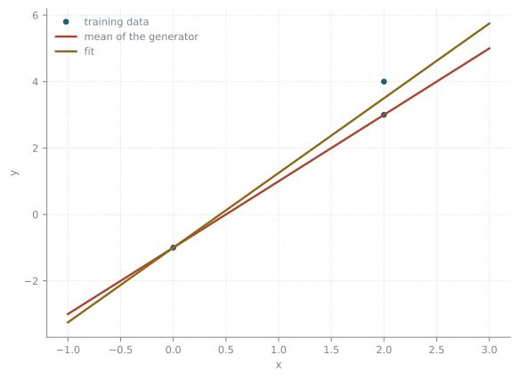

Figure 8.1: Three training points, the true mean of the data generating process, and the fitted line.

Four different losses

Training loss. The average loss on the data we fitted on.

Test loss at \(x_0\) for the conditional process. The expected loss under \(P(Y|x_0)\), at one fixed input.

Test loss for the joint process. The expected loss under \(P(X, Y)\). This is what we would like to make small. We usually do not know \(P(X, Y)\).

Test loss on a test set. The average loss on data from the same process that we did not use for fitting. This is an approximation of the previous one.

The generator below has a noise that grows with \(x\),

\[ Y = 2x - 1 + \Sigma(x)\,Z, \qquad \Sigma(x) = \Sigma_{\text{slope}}\,x + \Sigma_0, \qquad X, Z \sim \mathcal N(0, 1). \]

Because we know the generator, the test loss at \(x_0\) and the test loss for the joint process can both be written in closed form, for any fitted function. They are exact numbers rather than estimates. Finding the two expressions is exercise 5, and the panel reports the fitted slope and intercept so that you can evaluate your own answer and compare it with the two monitors.

The four losses of a linear fit. Two are measured on data, on the training set and on the test set; two are exact expectations, at \(x_0\) and over the joint process. The shaded band is \(\pm\Sigma(x)\) and the lobe at \(x_0\) is \(P(Y|x_0)\). With few training points the training loss sits far below the rest. As \(n\) grows all four settle down, and as \(N\) grows the test set loss converges on the joint loss it is estimating. Moving \(x_0\) alone changes only one of the four, and where it is large is worth watching before you do exercise 5.

Note that the training loss is usually smaller than the test loss. The parameters were chosen to make the training loss small, so some of the noise in the training set has been fitted as if it were signal.

Which loss should we use

The squared error is not always right. In a classification problem it makes little sense. And if we know something about the noise, we would like the loss to reflect that.

All of these questions have a clean answer if we start from a family of probability distributions instead of a family of functions. That is the next page.