Poisson regression

Examples

When the response is a count, a normal distribution is the wrong model. Counts are never negative, and their spread grows with their mean.

The model

We take \(Y|x \sim \mathrm{Poisson}(\lambda(x))\) with

\[ \lambda(x) = \exp(\beta_0 + \beta_1 x_1 + \cdots + \beta_p x_p). \]

The exponential keeps \(\lambda\) positive. It also makes the effects multiplicative. A coefficient of 0.1 means that a one unit increase in that predictor multiplies the expected count by \(e^{0.1} \approx 1.1\).

For a Poisson distribution the variance equals the mean. So the model does not have a separate noise parameter, and it predicts more spread where it predicts larger counts.

The Poisson distribution on its own. The single parameter sets both the mean and the spread, which is why the shape changes as it moves.

The rate is the exponential of a linear function, so it can never be negative. The band is one square root of the mean, which is the Poisson standard deviation. There is no separate σ to move.

Fitting

import numpy as np
import pandas as pd
from sklearn.linear_model import PoissonRegressor, LinearRegression

rng = np.random.default_rng(11)

n = 500
temp = rng.uniform(-5, 30, n)
humidity = rng.uniform(0.2, 1.0, n)
lam = np.exp(1.5 + 0.09 * temp - 1.6 * humidity)
count = rng.poisson(lam)

X = np.column_stack([temp, humidity])

pois = PoissonRegressor(alpha=0.0).fit(X, count)
lin = LinearRegression().fit(X, count)

print("intercept:", round(float(pois.intercept_), 3))
print("coefs:    ", pois.coef_.round(3))

1

alpha is the regularization constant. We set it to zero here to get the plain maximum likelihood fit.

intercept: 1.508
coefs:     [ 0.089 -1.58 ]

The fitted coefficients are close to the ones we used to generate the data.

Why not linear regression

import matplotlib.pyplot as plt

fig, ax = plt.subplots()
ax.plot(count, lin.predict(X), ".", alpha=0.4, label="linear regression")
ax.plot(count, pois.predict(X), ".", alpha=0.4, label="Poisson regression")
lim = [0, count.max() * 1.05]
ax.plot(lim, lim, ls="--", lw=1, color="#7a838b")
ax.set(xlabel="true count", ylabel="predicted count", xlim=lim, ylim=lim)
ax.legend()
plt.show()

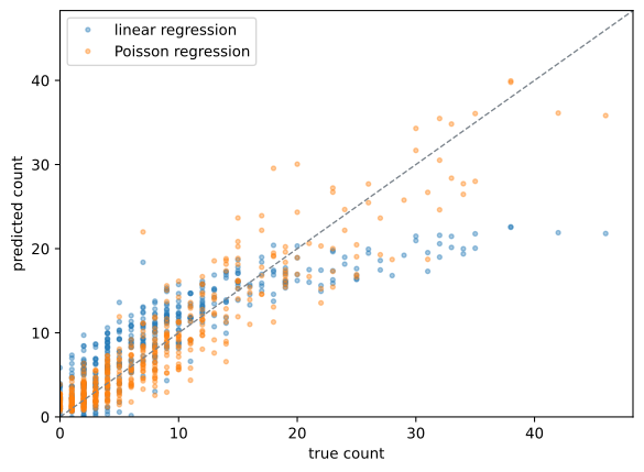
Figure 16.1: True counts against predictions. Points on the diagonal are perfect predictions.

print("negative predictions, linear: ", int((lin.predict(X) < 0).sum()))
print("negative predictions, Poisson:", int((pois.predict(X) < 0).sum()))

negative predictions, linear:  68
negative predictions, Poisson: 0

Linear regression predicts negative counts. It also puts equal weight on an error of 10 counts whether the true value is 5 or 500, which is not what we want.

Heteroscedasticity

pred = pois.predict(X)

fig, ax = plt.subplots()
ax.plot(pred, count - pred, ".", alpha=0.4)
ax.axhline(0, color="#a8452f", lw=1.2, ls="--")
ax.set(xlabel="predicted count", ylabel="residual")
plt.show()

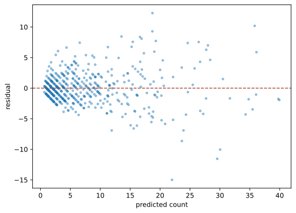
Figure 16.2: Residuals against the predicted count. The spread grows with the prediction, which is what a Poisson model expects.

For a normal model this plot would be a warning sign. For a Poisson model it is exactly what we expect, since the variance equals the mean.

If the spread is larger than the mean, the data is overdispersed. A negative binomial model is then a better choice.

What comes later

In week 8 we keep this likelihood and replace the linear predictor by a neural network,

\[ \lambda(x) = \exp(f_\theta(x)). \]

Nothing about the likelihood changes. Only the shape of \(\eta\) does.