In this example we generate data, write \(K\)-fold cross-validation from scratch, and use it to select a polynomial degree.
Setup
import numpy as npimport matplotlib.pyplot as pltRNG = np.random.default_rng(322)SIGMA =0.15def f(x):return np.sin(2* x) +2* (x -0.5) **3-0.5* xdef sample(n, rng=RNG): x = rng.uniform(0, 1, n)return x, f(x) + rng.normal(0, SIGMA, n)x, y = sample(80)print(f"n = {len(x)}, x in [{x.min():.2f}, {x.max():.2f}], y in [{y.min():.2f}, {y.max():.2f}]")
n = 80, x in [0.00, 0.97], y in [-0.30, 1.00]
Fitting a polynomial
Polynomial regression is linear regression on a transformed design matrix. The model is non-linear in \(x\), but it is linear in the parameters, so least squares applies without any change.
The columns are \(1, x, x^2, \dots, x^d\). This is the design matrix \(X\).
2
lstsq solves the normal equations \(X^\top X\beta = X^\top y\) in a stable way. Do not form \((X^\top X)^{-1}\) yourself.
coefficients: [-0.279  3.238 -4.031  1.718]
training MSE: 0.0239
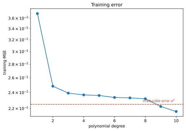
The training MSE always falls when we increase the degree. So we cannot use it to pick the degree. This is the whole problem.
degrees = np.arange(1, 11)train_err = [mse(fit(x, y, d), x, y) for d in degrees]fig, ax = plt.subplots()ax.plot(degrees, train_err, "o-")ax.axhline(SIGMA**2, ls="--", lw=1.2, color="#a8452f")ax.annotate("irreducible error $\\sigma^2$", (degrees[-1], SIGMA**2), xytext=(-4, 6), textcoords="offset points", ha="right", color="#a8452f", fontsize=8.5)ax.set(xlabel="polynomial degree", ylabel="training MSE", yscale="log")ax.set_title("Training error")plt.show()
Figure 26.1: The training error falls monotonically with flexibility.
\(K\)-fold cross-validation
def kfold_indices(n, K, rng=RNG):"""Shuffle, then cut into K blocks of nearly equal size."""return np.array_split(rng.permutation(n), K)def cross_val_mse(x, y, degree, K=10, rng=RNG): folds = kfold_indices(len(x), K, rng) total, count =0.0, 0for i inrange(K): val = folds[i] train = np.concatenate([folds[j] for j inrange(K) if j != i]) coef = fit(x[train], y[train], degree) total += mse(coef, x[val], y[val]) *len(val) count +=len(val)return total / countprint("10-fold CV MSE, degree 3:", round(cross_val_mse(x, y, 3), 4))
1
Fold i is held out. Everything else is used for training.
2
We refit inside the loop. A model that is fitted once outside the loop has seen every fold. This is the most common mistake here.
3
We weight by fold size, so that unequal folds do not skew the average.
10-fold CV MSE, degree 3: 0.0261
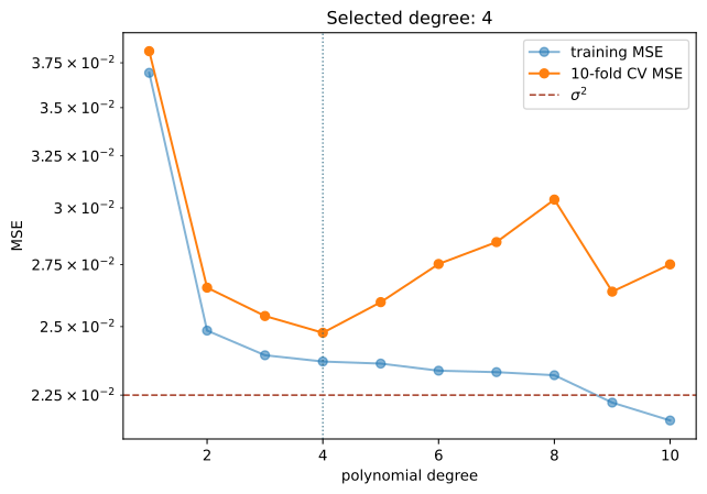
Now we run this for every degree and take the smallest.
cv_err = [cross_val_mse(x, y, d, K=10) for d in degrees]best = degrees[int(np.argmin(cv_err))]print(f"selected degree: {best} CV MSE: {min(cv_err):.4f}")
Figure 26.2: Cross-validated error and training error. The CV curve turns up where the extra flexibility costs more in variance than it gains in bias.
The same thing with scikit-learn
In practice we do not write the loop ourselves. Note that the model and the polynomial transformation go into one Pipeline, so that the transformation is also fitted inside each fold.
from sklearn.linear_model import LinearRegressionfrom sklearn.model_selection import KFold, cross_val_scorefrom sklearn.pipeline import make_pipelinefrom sklearn.preprocessing import PolynomialFeaturesX = x.reshape(-1, 1)cv = KFold(10, shuffle=True, random_state=0)scores = []for d in degrees: model = make_pipeline(PolynomialFeatures(d), LinearRegression()) s = cross_val_score(model, X, y, cv=cv, scoring="neg_mean_squared_error") scores.append(-s.mean())print("selected degree:", degrees[int(np.argmin(scores))])
selected degree: 4
Leave-one-out without fitting \(n\) times
For a model that is linear in its parameters the leave-one-out error has a closed form. We fit once, read the diagonal of the hat matrix, and divide.
def loocv_mse(x, y, degree): X = design(x, degree) Q, _ = np.linalg.qr(X) h = np.sum(Q**2, axis=1) coef, *_ = np.linalg.lstsq(X, y, rcond=None) resid = y - X @ coefreturnfloat(np.mean((resid / (1- h)) **2))loo = [loocv_mse(x, y, d) for d in degrees]print("LOOCV selects degree:", degrees[int(np.argmin(loo))])print("brute force check (degree 3):",round(cross_val_mse(x, y, 3, K=len(x)), 6), "vs", round(loocv_mse(x, y, 3), 6))
1
\(h_{ii}\) is the leverage of point \(i\). From the QR factorisation it is the squared row norm of \(Q\), so we never form \(H\) itself.
2
The residuals are inflated by \(1/(1-h_{ii})\). Points with high leverage are the ones the model would miss most if we removed them.
LOOCV selects degree: 3
brute force check (degree 3): 0.025934 vs 0.025934
The two numbers agree to six digits. That is the point of the check. The identity is exact, not an approximation.
What this page does not tell us
The value min(cv_err) above is not an estimate of the test error of the selected model. It is the smallest of ten correlated noisy numbers, and we chose it because it was small. See nested cross-validation.
The panel below makes the same point in a different way. Nothing changes except the shuffle.
The same data, the same models, only the shuffle changes. With a single split the chosen degree jumps around. With 10-fold it is far steadier.