Cleaning and feature engineering

Examples

Before we fit anything, the raw data has to be turned into a table of numbers. The choices we make here usually matter more than the choice of model.

Missing data

import numpy as np
import pandas as pd

datam = pd.DataFrame({
    "age": [12., 41, np.nan, 33, 27, 50],
    "gender": pd.Categorical([None, "female", "male", "male", "male", "female"]),
})
datam
age gender
0 12.0 NaN
1 41.0 female
2 NaN male
3 33.0 male
4 27.0 male
5 50.0 female

The simplest option is to drop the rows. This is fine if only a few rows are affected. It is not fine if the values are missing for a reason, because then the remaining rows are no longer a random sample.

datam.dropna()
age gender
1 41.0 female
3 33.0 male
4 27.0 male
5 50.0 female

The other option is to fill the missing values in. Note that the imputer learns the value it fills in, so it belongs inside the fold.

from sklearn.impute import SimpleImputer

imp = SimpleImputer(strategy="most_frequent")
pd.DataFrame(imp.fit_transform(datam), columns=["age", "gender"])
age gender
0 12.0 male
1 41.0 female
2 12.0 male
3 33.0 male
4 27.0 male
5 50.0 female

Removing useless predictors

A predictor with zero variance carries no information. Two predictors with correlation 1 carry the same information twice, which makes the least squares solution non-unique.

df = pd.DataFrame({"a": np.ones(5),
                   "b": np.random.randn(5),
                   "c": np.linspace(1, 5, 5),
                   "d": np.linspace(2, 10, 5),
                   "e": np.zeros(5)})

df = df.loc[:, np.std(df, axis=0) != 0]

corr = np.triu(df.corr().values, k=0)
np.fill_diagonal(corr, 0)
df = df.drop(df.columns[np.where(corr == 1)[1]], axis=1)
df
1
Columns a and e are constant.
2
Column d is 2 * c, so it is dropped.
b c
0 -1.713154 1.0
1 -0.002421 2.0
2 -0.866783 3.0
3 -0.154579 4.0
4 0.763934 5.0

Standardization

Standardization shifts the data so that the mean is 0 and scales it so that the standard deviation is 1. Some methods need it, for example regularization and \(k\) nearest neighbours. Others do not care.

from sklearn.preprocessing import StandardScaler

height_weight = pd.DataFrame({"height": [165., 175, 183, 152, 171],
                              "weight": [60., 71, 89, 47, 70]})

scaled = pd.DataFrame(StandardScaler().fit_transform(height_weight),
                      columns=["height", "weight"])
scaled.round(3)
height weight
0 -0.404 -0.535
1 0.558 0.260
2 1.327 1.561
3 -1.654 -1.474
4 0.173 0.188

The scaler learns the mean and the standard deviation from the data. If we fit it on all the data before splitting, the validation fold has already influenced the training set. Use a Pipeline.

Categorical predictors

A model cannot use the string "female". One-hot coding turns each category into its own column of zeros and ones.

from sklearn.preprocessing import OneHotEncoder

cdata = pd.DataFrame({
    "gender": pd.Categorical(["male", "male", "female", "female", "female", "male"]),
    "treatment": pd.Categorical([1, 2, 2, 1, 3, 2])})

enc = OneHotEncoder(sparse_output=False)
pd.DataFrame(enc.fit_transform(cdata),
             columns=enc.get_feature_names_out())
gender_female gender_male treatment_1 treatment_2 treatment_3
0 0.0 1.0 1.0 0.0 0.0
1 0.0 1.0 0.0 1.0 0.0
2 1.0 0.0 0.0 1.0 0.0
3 1.0 0.0 1.0 0.0 0.0
4 1.0 0.0 0.0 0.0 1.0
5 0.0 1.0 0.0 1.0 0.0

With an intercept in the model, one of the columns per category is redundant. The sum of all columns of one category is always 1, which is the intercept again. We therefore drop one column per category.

enc = OneHotEncoder(drop="first", sparse_output=False)
enc.fit_transform(cdata)
array([[1., 0., 0.],
       [1., 1., 0.],
       [0., 1., 0.],
       [0., 0., 0.],
       [0., 0., 1.],
       [1., 1., 0.]])

In a real data set only some columns are categorical, so we apply the encoder to those columns only.

from sklearn.compose import make_column_transformer
from sklearn.linear_model import LinearRegression
from sklearn.pipeline import Pipeline

wage = pd.DataFrame({
    "EDUCATION": [8, 9, 12, 12, 16, 18, 12, 14],
    "EXPERIENCE": [21, 42, 1, 4, 17, 9, 30, 6],
    "SEX": ["female", "male", "male", "female", "male", "female", "male", "female"],
    "UNION": ["not", "not", "not", "union", "union", "not", "union", "not"],
    "WAGE": [5.1, 4.9, 6.7, 4.0, 15.0, 22.2, 8.1, 9.4]})

categorical = ["SEX", "UNION"]

pre = make_column_transformer(
    (OneHotEncoder(drop="first"), categorical),
    remainder="passthrough",
    verbose_feature_names_out=False)

pipe = Pipeline([("encoder", pre), ("regressor", LinearRegression())])
pipe.fit(wage.drop("WAGE", axis=1), wage["WAGE"])

pd.DataFrame({"predictor": pipe[:-1].get_feature_names_out(),
              "coefficient": pipe[-1].coef_.round(3)})
predictor coefficient
0 SEX_male -1.233
1 UNION_union -2.792
2 EDUCATION 2.035
3 EXPERIENCE 0.157

Splines

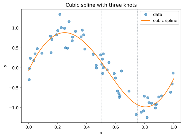
Polynomials are one way to make a linear model flexible, but a polynomial of high degree behaves badly at the edges of the data. Splines are piecewise polynomials that are joined at a set of knots, and they behave much better.

def spline_features(x, degree, knots):
    """Columns x, x^2, ..., x^degree, then one hinge per knot."""
    cols = [x ** d for d in range(1, degree + 1)]
    cols += [np.maximum(0, x - k) ** degree for k in knots]
    return np.column_stack(cols)


x = np.linspace(0, 1, 200)
H = spline_features(x, degree=3, knots=[0.25, 0.5, 0.75])
print("shape:", H.shape)
shape: (200, 6)
import matplotlib.pyplot as plt

rng = np.random.default_rng(7)
xs = rng.uniform(0, 1, 60)
ys = np.sin(6 * xs) + rng.normal(0, 0.25, 60)

knots = [0.25, 0.5, 0.75]
A = np.column_stack([np.ones_like(xs), spline_features(xs, 3, knots)])
beta, *_ = np.linalg.lstsq(A, ys, rcond=None)

grid = np.linspace(0, 1, 300)
G = np.column_stack([np.ones_like(grid), spline_features(grid, 3, knots)])

fig, ax = plt.subplots()
ax.plot(xs, ys, "o", alpha=0.6, label="data")
ax.plot(grid, G @ beta, label="cubic spline")
for k in knots:
    ax.axvline(k, color="#7a838b", lw=0.7, ls=":")
ax.set(xlabel="x", ylabel="y")
ax.set_title("Cubic spline with three knots")
ax.legend()
plt.show()
Figure 28.1: A cubic spline fitted to noisy data, with three knots.

sklearn has SplineTransformer, which uses a better basis than the one above but does the same thing.

Move the knots and the degree. The fit is refitted in the browser each time. Note how little a degree 1 spline needs in order to follow the curve, and how a knot placed in a flat region does almost nothing.

Transforming the output

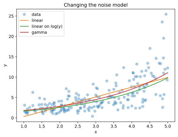
Sometimes the response itself is the problem. If the response is positive and its spread grows with its mean, a linear model with normal noise is the wrong model.

There are two ways out. We can take the logarithm of the response and fit a linear model. Or we can keep the response and change the noise model, for example to a Gamma or a Poisson distribution.

from sklearn.linear_model import GammaRegressor, LinearRegression

rng = np.random.default_rng(1)
X = rng.uniform(1, 5, (200, 1))
y = rng.gamma(shape=4.0, scale=np.exp(0.5 * X[:, 0]) / 4.0)

lin = LinearRegression().fit(X, y)
log = LinearRegression().fit(X, np.log(y))
gam = GammaRegressor(alpha=0.0).fit(X, y)

grid = np.linspace(1, 5, 100).reshape(-1, 1)
print("linear at x=5:      ", round(float(lin.predict([[5.0]])[0]), 2))
print("log-linear at x=5:  ", round(float(np.exp(log.predict([[5.0]])[0])), 2))
print("gamma at x=5:       ", round(float(gam.predict([[5.0]])[0]), 2))
linear at x=5:       9.94
log-linear at x=5:   9.81
gamma at x=5:        11.08
fig, ax = plt.subplots()
ax.plot(X[:, 0], y, "o", alpha=0.35, label="data")
ax.plot(grid, lin.predict(grid), label="linear")
ax.plot(grid, np.exp(log.predict(grid)), label="linear on log(y)")
ax.plot(grid, gam.predict(grid), label="gamma")
ax.set(xlabel="x", ylabel="y")
ax.set_title("Changing the noise model")
ax.legend()
plt.show()
Figure 28.2: Three models for a positive response whose spread grows with its mean.

The two are not the same. A linear model on \(\log y\) models the mean of \(\log y\), and \(\exp\) of that is not the mean of \(y\). The Gamma model works with \(y\) directly.

A recipe

  1. Collect data.
  2. Look at the raw data and clean it.
  3. Choose a representation of the raw data.
  4. Choose a method.
  5. Fit and tune the hyper-parameters with cross-validation.
  6. If the training loss is high and the test loss is high, take a more flexible method. If the training loss is low and the test loss is high, take a less flexible method.
  7. Repeat 4 to 6.
  8. If still unhappy, go back to 2, or collect more data.
  9. Fit the best model on all available data.