import numpy as np
import torch
import matplotlib.pyplot as plt

torch.manual_seed(6)

n = 400
X = torch.randn(n, dtype=torch.float64)
y = 0.1 - 0.4 * X + 0.3 * torch.randn(n, dtype=torch.float64)


def run(batch_size, eta, epochs=30):
    beta = torch.tensor([1.5, 1.5], requires_grad=True)
    curve = []
    steps_per_epoch = max(1, n // batch_size)
    for _ in range(epochs):
        perm = torch.randperm(n)
        for s in range(steps_per_epoch):
            idx = perm[s * batch_size:(s + 1) * batch_size]
            loss = torch.mean((y[idx] - beta[0] - beta[1] * X[idx]) ** 2)
            loss.backward()
            with torch.no_grad():
                beta -= eta * beta.grad
            beta.grad.zero_()
        with torch.no_grad():
            curve.append(float(torch.mean((y - beta[0] - beta[1] * X) ** 2)))
return np.array(curve)Stochastic gradient descent
Examples
Computing the gradient of the full training loss means going through all \(n\) points for every single step. With a million points that is too slow.
Instead we compute the gradient on a small random subset, called a batch, and take a step. The gradient is then noisy, but we get many more steps for the same work.
Terminology
A batch is a subset of the training data used for one step. The batch size is how many points are in it. An epoch is one pass through the whole training set, so \(n / \text{batch size}\) steps.
With a batch size of 1 this is called stochastic gradient descent. With a batch size equal to \(n\) it is ordinary gradient descent. In practice we use something in between, often 32 or 128.
An example
The full-batch curve is smooth but it moves slowly, because it takes one step per epoch. The small batches take many steps per epoch and get there much faster, at the cost of a noisy curve.
Using an optimizer
torch has optimizers that take care of the update rule. Adam adapts the learning rate per parameter and usually needs less tuning than plain gradient descent.
def advanced_gradient_descent(loss, x, optimizer, T):
    curve = []
    for t in range(T):
        optimizer.zero_grad()
        l = loss(x)
        l.backward()
        optimizer.step()
        curve.append(float(l))
    return x, np.array(curve)


beta = torch.tensor([1.5, 1.5], requires_grad=True)
opt = torch.optim.Adam([beta], lr=0.05)
beta, curve = advanced_gradient_descent(
    lambda b: torch.mean((y - b[0] - b[1] * X) ** 2), beta, opt, 400)

print("Adam:", beta.detach().numpy().round(4))
Adam: [ 0.1071 -0.3822]Learning curves
Always plot the learning curve. It answers two questions at once.
If the curve is still going down at the end, we stopped too early. Train longer.
If the curve fluctuates wildly at the end, the learning rate is too large. Lower it.
Use a log scale on the vertical axis. Otherwise the interesting part at the end is invisible.
Early stopping
If we also track the loss on a validation set, we usually see it fall, reach a minimum, and rise again. The model has started to fit the noise in the training set.
Stopping at the minimum of the validation curve is called early stopping. It is a form of regularization. The number of steps plays the same role that \(\lambda\) played for ridge regression, and for a linear model the two are approximately equivalent.
from sklearn.linear_model import Ridge
from sklearn.preprocessing import PolynomialFeatures

rng = np.random.default_rng(6)
xs = rng.uniform(0, 1, 30)
ys = np.sin(6 * xs) + rng.normal(0, 0.3, 30)
xv = rng.uniform(0, 1, 300)
yv = np.sin(6 * xv) + rng.normal(0, 0.3, 300)

P = PolynomialFeatures(14)
A = torch.tensor(P.fit_transform(xs.reshape(-1, 1)))
Av = torch.tensor(P.transform(xv.reshape(-1, 1)))
t = torch.tensor(ys)
tv = torch.tensor(yv)

w = torch.zeros(A.shape[1], dtype=torch.float64, requires_grad=True)
opt = torch.optim.SGD([w], lr=1e-3)
tr, va = [], []
for step in range(4000):
    opt.zero_grad()
    l = torch.mean((A @ w - t) ** 2)
    l.backward()
    opt.step()
    tr.append(float(l))
    with torch.no_grad():
        va.append(float(torch.mean((Av @ w - tv) ** 2)))

best = int(np.argmin(va))
fig, ax = plt.subplots()
ax.plot(tr, label="training")
ax.plot(va, label="validation")
ax.axvline(best, color="#a8452f", ls="--", lw=1.2, label=f"stop at {best}")
ax.set(xlabel="step", ylabel="loss", yscale="log")
ax.legend()
plt.show()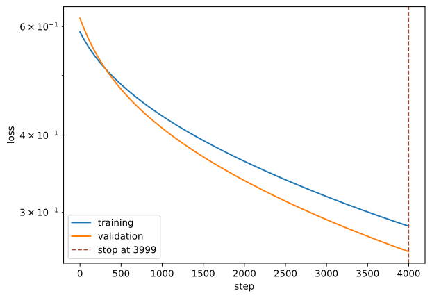
Feature engineering, automated
The XOR problem is the classic example of a data set that no linear model can solve. The two classes are not linearly separable.
We can solve it by hand, by adding the product \(x_1 x_2\) as a feature. That works, but it required us to know the answer.
The alternative is to let the machine find the features. That is what a neural network does, and it is the subject of week 7.