Building networks

Examples

A network in torch

import numpy as np
import torch
import matplotlib.pyplot as plt

torch.manual_seed(7)

net = torch.nn.Sequential(
    torch.nn.Linear(3, 30),
    torch.nn.ReLU(),
    torch.nn.Linear(30, 2),
)

n_params = sum(p.numel() for p in net.parameters())
print(net)
print("parameters:", n_params)

1

From 3 inputs to 30 hidden neurons. This layer has \(30 \times 4 = 120\) parameters.

2

From 30 hidden neurons to 2 outputs, so \(2 \times 31 = 62\) parameters.

Sequential(
  (0): Linear(in_features=3, out_features=30, bias=True)
  (1): ReLU()
  (2): Linear(in_features=30, out_features=2, bias=True)
)
parameters: 182

x = torch.rand(3)
net(x).detach().numpy().round(4)

array([0.1888, 0.0847], dtype=float32)

Different activation functions can be mixed, although in practice we rarely do.

net2 = torch.nn.Sequential(
    torch.nn.Linear(20, 100), torch.nn.ReLU(),
    torch.nn.Linear(100, 50), torch.nn.Tanh(),
    torch.nn.Linear(50, 10),
)
net2(torch.rand(20)).detach().numpy().round(3)

array([-0.224, -0.186, -0.076, -0.175,  0.176,  0.062,  0.159, -0.106,
       -0.32 , -0.098], dtype=float32)

What one hidden layer can do

A relu network with one hidden layer is a piecewise linear function. Each neuron contributes a kink.

A network with one hidden layer of relu neurons, fitted to the same 60 points. Switch to the hidden units to see the individual pieces that are summed to make the fit. Each neuron contributes one kink.

Fitting a regression

We fit the weather data. Note the two things we do before training. We standardize the input, and we standardize the output as well, which makes the default learning rate work.

import pandas as pd
from sklearn.preprocessing import StandardScaler

weather = pd.read_csv("https://go.epfl.ch/bio322-weather2015-2018.csv")
Xdf = weather.iloc[:-5].drop(columns=["LUZ_wind_peak", "time"])
ydf = weather["LUZ_wind_peak"][5:].values

xs, ys = StandardScaler(), StandardScaler()
Xn = xs.fit_transform(Xdf.values)
yn = ys.fit_transform(ydf.reshape(-1, 1))

Xt = torch.tensor(Xn, dtype=torch.float32)
yt = torch.tensor(yn, dtype=torch.float32)

model = torch.nn.Sequential(
    torch.nn.Linear(Xt.shape[1], 128), torch.nn.ReLU(),
    torch.nn.Linear(128, 64), torch.nn.ReLU(),
    torch.nn.Linear(64, 1),
)

opt = torch.optim.Adam(model.parameters(), lr=1e-3)
loader = torch.utils.data.DataLoader(
    torch.utils.data.TensorDataset(Xt, yt), batch_size=128, shuffle=True)

curve = []
for epoch in range(15):
    for xb, yb in loader:
        opt.zero_grad()
        loss = torch.mean((model(xb) - yb) ** 2)
        loss.backward()
        opt.step()
    with torch.no_grad():
        curve.append(float(torch.mean((model(Xt) - yt) ** 2)))

print("training MSE on standardized output:", round(curve[-1], 4))

1

The scaler is fitted on the training data only. In a real analysis this goes inside the cross-validation fold.

2

The output layer is linear, because the response is continuous.

training MSE on standardized output: 0.39

fig, ax = plt.subplots()
ax.plot(curve, "o-")
ax.set(xlabel="epoch", ylabel="training MSE", yscale="log")
plt.show()

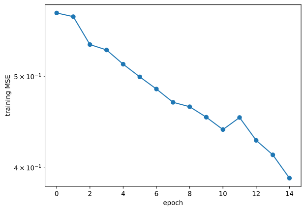
Figure 36.1: The learning curve. It is flat at the end, so more epochs would not help much.

To get predictions in the original units we invert the output scaler.

with torch.no_grad():
    pred = ys.inverse_transform(model(Xt).numpy())
rmse = float(np.sqrt(np.mean((pred[:, 0] - ydf) ** 2)))
print("training RMSE in km/h:", round(rmse, 3))

training RMSE in km/h: 6.462

Compare this to the linear regression from week 2. The network fits the training data better. Whether it predicts better is a different question, and we would answer it with cross-validation.

The same thing with scikit-learn

For small problems MLPRegressor is quicker to write. It has fewer options than torch, which is often an advantage.

from sklearn.neural_network import MLPRegressor

m = MLPRegressor(hidden_layer_sizes=(128, 64), max_iter=200)
m.fit(Xn, ydf)