Four methods on one data set

Examples

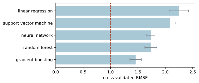
We now have several methods. This page compares them on one data set, scored the same way.

This is what the project asks for, so it is worth reading closely.

The data

import numpy as np
import pandas as pd
from sklearn.model_selection import train_test_split

rng = np.random.default_rng(10)
n, p = 1200, 12

X = rng.normal(0, 1, (n, p))
y = (3 * X[:, 0]
     - 2 * X[:, 1]
     + 1.5 * X[:, 0] * X[:, 2]
     + 2 * np.sin(2 * X[:, 3])
     + rng.normal(0, 1.0, n))

Xtr, Xte, ytr, yte = train_test_split(X, y, test_size=0.3, random_state=0)
print("train:", Xtr.shape, " test:", Xte.shape)

1: Two predictors enter linearly.
2: One interaction.
3: One non-linear term. The remaining eight predictors are noise.

train: (840, 12)  test: (360, 12)

The models

Every model goes into a Pipeline with a scaler, so that the scaling is fitted inside each fold and not on the whole data set.

from sklearn.ensemble import RandomForestRegressor, GradientBoostingRegressor
from sklearn.linear_model import LinearRegression
from sklearn.model_selection import KFold, cross_val_score
from sklearn.neural_network import MLPRegressor
from sklearn.pipeline import make_pipeline
from sklearn.preprocessing import StandardScaler
from sklearn.svm import SVR

models = {
    "linear regression": make_pipeline(StandardScaler(), LinearRegression()),
    "random forest": make_pipeline(StandardScaler(),
                                   RandomForestRegressor(n_estimators=300, random_state=0)),
    "gradient boosting": make_pipeline(StandardScaler(),
                                       GradientBoostingRegressor(random_state=0)),
    "support vector machine": make_pipeline(StandardScaler(), SVR(C=10, gamma="scale")),
    "neural network": make_pipeline(StandardScaler(),
                                    MLPRegressor(hidden_layer_sizes=(64, 64),
                                                 max_iter=1500, random_state=0)),
}

Cross-validating on the training set

cv = KFold(5, shuffle=True, random_state=0)

rows = []
for name, m in models.items():
    s = cross_val_score(m, Xtr, ytr, cv=cv, scoring="neg_root_mean_squared_error")
    rows.append({"model": name, "CV RMSE": round(-s.mean(), 3), "sd": round(s.std(), 3)})

table = pd.DataFrame(rows).sort_values("CV RMSE")
table

	model	CV RMSE	sd
2	gradient boosting	1.459	0.107
1	random forest	1.736	0.111
4	neural network	1.737	0.076
3	support vector machine	2.088	0.093
0	linear regression	2.252	0.171

Note the standard deviation column. If two models differ by less than the spread across folds, we cannot tell them apart on this data.

import matplotlib.pyplot as plt

fig, ax = plt.subplots(figsize=(6.0, 2.8))
ax.barh(table["model"], table["CV RMSE"], xerr=table["sd"],
        color="#a8c8d6", error_kw={"ecolor": "#7a838b", "capsize": 3})
ax.axvline(1.0, ls="--", lw=1.2, color="#a8452f")
ax.set(xlabel="cross-validated RMSE")
plt.show()

Figure 52.1: Cross-validated RMSE with the spread across folds. The dashed line is the noise level, which no model can beat.

Scoring the winner once

from sklearn.metrics import mean_squared_error

best_name = table.iloc[0]["model"]
best = models[best_name].fit(Xtr, ytr)
rmse = mean_squared_error(yte, best.predict(Xte)) ** 0.5

print(f"selected model: {best_name}")
print(f"test RMSE:      {rmse:.3f}")

1: The test set has not been touched until this line. It was not used to choose the model and not used to tune anything.

selected model: gradient boosting
test RMSE:      1.431

The cross-validated score of the winner is optimistic, because we chose the winner with it. The test score is the honest number. It is usually a little worse, and that is expected.

What to take from this

The linear model misses the interaction and the non-linear term, so it is clearly worse. The tree ensembles find both without being told about them.

Try a simple model first. It is fast, it is a baseline, and sometimes it wins.

Score everything the same way, on the same folds. Comparing a number from one paper with a number from another is almost never meaningful.

Report the test score, not the cross-validated one.