Counts

Examples

The last row of the table. The response is a count, so the distribution is Poisson, the output layer is \(\exp\), and the loss is the negative Poisson log-likelihood.

\[ Y|x \sim \mathrm{Poisson}(\lambda(x)), \qquad \lambda(x) = e^{\eta}. \]

The rate is the exponential of a linear function, so it can never be negative. The band is one square root of the mean, which is the Poisson standard deviation. There is no separate σ to move.

Fitting, with a linear \(\eta\)

import numpy as np
import pandas as pd
import torch
import matplotlib.pyplot as plt
from sklearn.linear_model import PoissonRegressor, LinearRegression
from sklearn.metrics import mean_poisson_deviance

rng = np.random.default_rng(11)
torch.manual_seed(11)

n = 2000
temp = rng.uniform(-5, 30, n)
humidity = rng.uniform(0.2, 1.0, n)
lam = np.exp(1.5 + 0.09 * temp - 1.6 * humidity)
count = rng.poisson(lam)

X = np.column_stack([temp, humidity])
Xtr, Xte = X[:1500], X[1500:]
ytr, yte = count[:1500], count[1500:]

pois = PoissonRegressor(alpha=0.0).fit(Xtr, ytr)
lin = LinearRegression().fit(Xtr, ytr)

print("intercept:", round(float(pois.intercept_), 3))
print("coefs:    ", pois.coef_.round(3))
1
alpha is the regularization constant. We set it to zero here to get the plain maximum likelihood fit.
intercept: 1.484
coefs:     [ 0.092 -1.634]

The fitted coefficients are close to the ones we used to generate the data, and they read multiplicatively: one degree warmer multiplies the expected count by \(e^{0.09} \approx 1.09\).

Why not linear regression

fig, ax = plt.subplots()
ax.plot(yte, lin.predict(Xte), ".", alpha=0.4, label="linear regression")
ax.plot(yte, pois.predict(Xte), ".", alpha=0.4, label="Poisson regression")
lim = [0, yte.max() * 1.05]
ax.plot(lim, lim, ls="--", lw=1, color="#7a838b")
ax.set(xlabel="true count", ylabel="predicted count", xlim=lim, ylim=lim)
ax.legend()
plt.show()
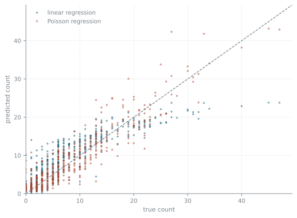
Figure 39.1: True counts against predictions. Points on the diagonal are perfect predictions.
print("negative predictions, linear: ", int((lin.predict(Xte) < 0).sum()))
print("negative predictions, Poisson:", int((pois.predict(Xte) < 0).sum()))
negative predictions, linear:  74
negative predictions, Poisson: 0

Linear regression predicts negative counts. It also puts equal weight on an error of 10 counts whether the true value is 5 or 500, which is not what we want. The wrong distribution is not a small mistake that a bigger model will absorb.

The same likelihood, with a learned \(\eta\)

Only \(\eta\) changes. The exponential and the loss are copied straight from the linear version.

class PoissonNet(torch.nn.Module):
    def __init__(self, p, hidden=32):
        super().__init__()
        self.body = torch.nn.Sequential(
            torch.nn.Linear(p, hidden), torch.nn.ReLU(),
            torch.nn.Linear(hidden, hidden), torch.nn.ReLU(),
            torch.nn.Linear(hidden, 1),
        )

    def forward(self, x):
        return torch.exp(self.body(x)).squeeze(-1)


def poisson_loss(rate, y):
    return torch.mean(rate - y * torch.log(rate + 1e-8))


mu, sd = Xtr.mean(0), Xtr.std(0)
Xtr_t = torch.tensor((Xtr - mu) / sd, dtype=torch.float32)
Xte_t = torch.tensor((Xte - mu) / sd, dtype=torch.float32)
ytr_t = torch.tensor(ytr, dtype=torch.float32)

net = PoissonNet(X.shape[1])
opt = torch.optim.Adam(net.parameters(), lr=1e-2)
loader = torch.utils.data.DataLoader(
    torch.utils.data.TensorDataset(Xtr_t, ytr_t), batch_size=64, shuffle=True)

for epoch in range(30):
    for xb, yb in loader:
        opt.zero_grad()
        poisson_loss(net(xb), yb).backward()
        opt.step()
1
The exponential is the inverse link, and it is the output layer. It keeps the rate positive.
2
The negative Poisson log-likelihood, dropping the \(\log y!\) term, which does not depend on the parameters. The small constant inside the log guards against a rate of exactly zero.
3
Standardization computed on the training part only. The linear model did not need it; gradient descent does.
with torch.no_grad():
    net_pred = net(Xte_t).numpy()

pd.DataFrame({
    "model": ["linear regression", "Poisson regression", "Poisson network"],
    "test deviance": [round(float(mean_poisson_deviance(yte, np.maximum(lin.predict(Xte), 1e-6))), 4),
                      round(float(mean_poisson_deviance(yte, pois.predict(Xte))), 4),
                      round(float(mean_poisson_deviance(yte, net_pred)), 4)],
})
model test deviance
0 linear regression 6.4360
1 Poisson regression 1.2410
2 Poisson network 1.2328

The network matches the Poisson regression and does not beat it. It should not: the data really was generated by an exponential of a linear function, so the linear model is exactly right and the network can only spend parameters rediscovering it.

That is the honest outcome to expect whenever the linear predictor is adequate, and it is why a ladder of models beginning with the simplest one is the right way to work.

Heteroscedasticity

pred = pois.predict(Xte)

fig, ax = plt.subplots()
ax.plot(pred, yte - pred, ".", alpha=0.4)
ax.axhline(0, color="#a8452f", lw=1.2, ls="--")
ax.set(xlabel="predicted count", ylabel="residual")
plt.show()
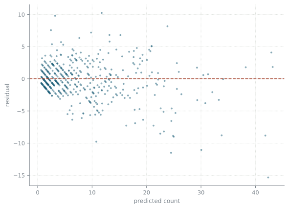
Figure 39.2: Residuals against the predicted count. The spread grows with the prediction, which is what a Poisson model expects.

For a normal model this plot would be a warning sign. For a Poisson model it is exactly what we expect, since the variance equals the mean.

If the spread is larger than the mean, the data is overdispersed. A negative binomial model is then a better choice.

What comes next

Week 8 takes this same pair of models to a real data set, where the linear predictor is not adequate, and where getting the features right turns out to matter more than either choice on this page.