import numpy as np
import pandas as pd
import matplotlib.pyplot as plt
from sklearn.linear_model import LogisticRegression
from sklearn.metrics import confusion_matrix, roc_curve, roc_auc_score

rng = np.random.default_rng(3)

n = 400
x = rng.normal(0, 2, n)
p = 1 / (1 + np.exp(-(0.9 * x - 0.4)))
y = (rng.random(n) < p).astype(int)

X = x.reshape(-1, 1)
m = LogisticRegression().fit(X, y)
prob = m.predict_proba(X)[:, 1]Evaluating a classifier
Examples
A classifier outputs a probability. A confusion matrix needs a decision. The step between the two is a threshold, and it is a choice.
Everything on this page applies to both columns of the grid. Nothing in it knows or cares whether \(\eta\) came from a linear function or from a network.
The confusion matrix
cm = confusion_matrix(y, (prob >= 0.5).astype(int))
pd.DataFrame(cm,
index=["true negative class", "true positive class"],
columns=["predicted negative", "predicted positive"])- 1
-
Note that
sklearnputs the true class in the rows and the predicted class in the columns. Many textbooks do it the other way round. Always check which convention a table uses before reading numbers off it.
| predicted negative | predicted positive | |
|---|---|---|
| true negative class | 156 | 47 |
| true positive class | 51 | 146 |
From the four counts we get the usual quantities.
tn, fp, fn, tp = cm.ravel()

pd.DataFrame({
    "quantity": ["accuracy", "sensitivity (recall, TPR)", "specificity (1 - FPR)",
                 "precision", "error rate"],
    "formula": ["(TP+TN)/all", "TP/(TP+FN)", "TN/(TN+FP)", "TP/(TP+FP)", "(FP+FN)/all"],
    "value": [round((tp + tn) / cm.sum(), 3),
              round(tp / (tp + fn), 3),
              round(tn / (tn + fp), 3),
              round(tp / (tp + fp), 3),
              round((fp + fn) / cm.sum(), 3)],
})| quantity | formula | value | |
|---|---|---|---|
| 0 | accuracy | (TP+TN)/all | 0.755 |
| 1 | sensitivity (recall, TPR) | TP/(TP+FN) | 0.741 |
| 2 | specificity (1 - FPR) | TN/(TN+FP) | 0.768 |
| 3 | precision | TP/(TP+FP) | 0.756 |
| 4 | error rate | (FP+FN)/all | 0.245 |
The threshold is a choice
Lowering the threshold predicts the positive class more often. That raises the true positive rate and the false positive rate at the same time.
Which error matters is a question about the application, not about the model. For a screening test a false negative may be far worse than a false positive. In that case we accept a lower threshold and more false alarms.
Note what the threshold does not change. The fitted parameters, the cross-entropy, and every probability the model outputs are all fixed before the threshold is chosen. Reporting a single accuracy hides that choice inside one number.
ROC and AUC
The ROC curve is what we get by sweeping the threshold from 1 to 0 and plotting the true positive rate against the false positive rate.
The area under the curve summarizes all thresholds in one number. It is the probability that a randomly chosen positive case gets a higher score than a randomly chosen negative case. A value of 0.5 means the classifier is useless and 1.0 means it separates the classes perfectly.
The AUC does not depend on the threshold, which makes it useful for comparing models. It also does not tell us which threshold to use, so it is not enough on its own.
Comparing two models honestly
Here is the quadrant problem from two pages back, scored properly rather than by a single accuracy at the default threshold.
import torch

torch.manual_seed(7)
rng = np.random.default_rng(7)

def make(n, rng):
    X = rng.uniform(-3, 3, (n, 2))
    eta = 1.4 * X[:, 0] * X[:, 1]
    return X.astype(np.float32), (rng.random(n) < 1 / (1 + np.exp(-eta))).astype(np.float32)

Xtr, ytr = make(600, rng)
Xte, yte = make(4000, rng)

lin = LogisticRegression(penalty=None).fit(Xtr, ytr)

net = torch.nn.Sequential(
    torch.nn.Linear(2, 32), torch.nn.ReLU(),
    torch.nn.Linear(32, 32), torch.nn.ReLU(),
    torch.nn.Linear(32, 1),
)
opt = torch.optim.Adam(net.parameters(), lr=1e-2)
loss_fn = torch.nn.BCEWithLogitsLoss()
loader = torch.utils.data.DataLoader(
    torch.utils.data.TensorDataset(torch.tensor(Xtr), torch.tensor(ytr).unsqueeze(1)),
    batch_size=64, shuffle=True)
for epoch in range(60):
    for xb, yb in loader:
        opt.zero_grad()
        loss_fn(net(xb), yb).backward()
        opt.step()

with torch.no_grad():
    score_net = torch.sigmoid(net(torch.tensor(Xte)).squeeze(1)).numpy()
score_lin = lin.predict_proba(Xte)[:, 1]
fig, ax = plt.subplots(figsize=(4.2, 4.0))
for score, label in [(score_lin, "logistic regression"), (score_net, "network")]:
fpr, tpr, _ = roc_curve(yte, score)
ax.plot(fpr, tpr, label=f"{label}, AUC = {roc_auc_score(yte, score):.3f}")
ax.plot([0, 1], [0, 1], ls="--", lw=1, color="#7a838b")
ax.set(xlabel="false positive rate", ylabel="true positive rate")
ax.legend(loc="lower right")
plt.show()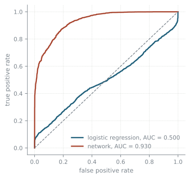
An AUC near 0.5 is not a badly tuned model. It is a model whose family cannot express the boundary, and no threshold rescues it. Compare that with the spam data on the classification page, where both AUCs are high and within a couple of points of each other. The same substitution, two very different verdicts, and only the data decides which one you get.
Imbalanced classes
If 97 percent of cases are negative, a model that always predicts negative has 97 percent accuracy. Accuracy is not a useful number here.
y_rare = np.zeros(1000, dtype=int)
y_rare[:30] = 1
always_negative = np.zeros(1000, dtype=int)

tn, fp, fn, tp = confusion_matrix(y_rare, always_negative).ravel()
print("accuracy:   ", round((tp + tn) / 1000, 3))
print("sensitivity:", round(tp / (tp + fn), 3))
accuracy: 0.97
sensitivity: 0.0Report sensitivity and precision, or the AUC, whenever the classes are imbalanced.
This is the same gap we met in week 2: the loss we fit is the cross-entropy, and the number we report is something else. Choosing that something else is part of stating the problem, not part of fitting it.