The data and the features

Examples

We want to predict how many bicycles are rented in a given hour in Washington DC.

The response is a count. It is never negative, and the spread grows with the mean. So the distribution is Poisson and not normal.

Loading

from sklearn.datasets import fetch_openml

bikes = fetch_openml(data_id=42712, as_frame=True, parser="auto").frame

To keep this page fast we use a small simulated version with the same structure.

import numpy as np
import pandas as pd

rng = np.random.default_rng(8)
n = 4000

hour = rng.integers(0, 24, n)
weekday = rng.integers(0, 7, n)
temp = rng.uniform(-4, 34, n)
humidity = rng.uniform(0.2, 1.0, n)
holiday = rng.random(n) < 0.05

# two commuter peaks on working days, one broad peak at the weekend
peak = np.where(weekday < 5,
                np.exp(-0.5 * ((hour - 8) / 1.3) ** 2) + np.exp(-0.5 * ((hour - 18) / 1.6) ** 2),
                0.9 * np.exp(-0.5 * ((hour - 14) / 4.0) ** 2))

rate = np.exp(2.0 + 1.6 * peak + 0.05 * temp - 1.3 * humidity - 0.4 * holiday)
count = rng.poisson(rate)

bikes = pd.DataFrame({"hour": hour, "weekday": weekday, "temp": temp,
                      "humidity": humidity, "holiday": holiday, "count": count})
bikes.head()

	hour	weekday	temp	humidity	holiday	count
0	17	1	32.472457	0.561865	False	57
1	7	0	21.624854	0.563670	False	37
2	5	5	7.567937	0.643465	False	3
3	23	0	5.075526	0.269698	False	7
4	4	1	1.199744	0.293597	False	3

Looking at the raw data

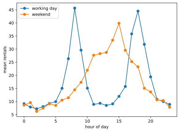
import matplotlib.pyplot as plt

fig, ax = plt.subplots()
for wd, label in [(bikes.weekday < 5, "working day"), (bikes.weekday >= 5, "weekend")]:
    m = bikes[wd].groupby("hour")["count"].mean()
    ax.plot(m.index, m.values, "o-", label=label)
ax.set(xlabel="hour of day", ylabel="mean rentals")
ax.legend()
plt.show()

Figure 40.1: Mean rentals per hour, split by working day and weekend.

Two peaks on working days, one broad peak at the weekend. A model that treats the hour as a single number cannot express this.

The features

The raw predictors need work.

Hour of day is not a number. Hour 23 is next to hour 0, but 23 is far from 0 on the number line. There are two ways to fix this. We can one-hot code the 24 hours, which gives the model complete freedom but 23 extra columns. Or we can use a cyclic encoding,

\[ \sin\left(\frac{2\pi h}{24}\right), \qquad \cos\left(\frac{2\pi h}{24}\right), \]

which uses two columns and puts hour 23 next to hour 0 where it belongs.

The same Poisson model with three encodings of the hour. As a plain number the model can only bend the curve once. The cyclic encoding captures the two commuter peaks with four columns. One-hot fits them exactly, with 23.

Weekday we one-hot code. Or, since the pattern is mostly working day against weekend, a single indicator may be enough.

Temperature and humidity we standardize.

from sklearn.compose import ColumnTransformer
from sklearn.preprocessing import OneHotEncoder, StandardScaler
from sklearn.pipeline import Pipeline


def add_cyclic(df):
    out = df.copy()
    out["hour_sin"] = np.sin(2 * np.pi * out["hour"] / 24)
    out["hour_cos"] = np.cos(2 * np.pi * out["hour"] / 24)
    out["working"] = (out["weekday"] < 5).astype(int)
    return out.drop(columns=["hour", "weekday"])


raw_features = ColumnTransformer([
    ("onehot", OneHotEncoder(drop="first", sparse_output=False), ["hour", "weekday", "holiday"]),
    ("scale", StandardScaler(), ["temp", "humidity"]),
])

X_raw = bikes.drop(columns=["count"])
y = bikes["count"].values

print("one-hot representation:", raw_features.fit_transform(X_raw).shape)
print("cyclic representation: ", add_cyclic(X_raw).shape)

one-hot representation: (4000, 32)
cyclic representation:  (4000, 6)

A ladder of models

Always start with a model that is hard to get wrong, and earn the complexity.

from sklearn.linear_model import PoissonRegressor
from sklearn.model_selection import KFold, cross_val_score

cv = KFold(5, shuffle=True, random_state=0)


def score(model, X):
    s = cross_val_score(model, X, y, cv=cv,
                        scoring="neg_mean_poisson_deviance")
    return -s.mean()


plain = Pipeline([("scale", StandardScaler()), ("glm", PoissonRegressor(max_iter=5000))])
onehot = Pipeline([("pre", raw_features), ("glm", PoissonRegressor(max_iter=5000))])

print(f"Poisson GLM, raw predictors:        {score(plain, X_raw.astype(float)):.3f}")
print(f"Poisson GLM, one-hot hour+weekday:  {score(onehot, X_raw):.3f}")
print(f"Poisson GLM, cyclic hour:           {score(plain, add_cyclic(X_raw).astype(float)):.3f}")

1

The Poisson deviance, not the squared error. We score with the same likelihood we fit with.

Poisson GLM, raw predictors:        6.427
Poisson GLM, one-hot hour+weekday:  4.543
Poisson GLM, cyclic hour:           5.634

The features matter more than the model here. Giving the model the hour in a usable form improves it far more than anything we will do in the next page.