We keep the Poisson likelihood from week 7 and replace the linear predictor by a network,
\[
\lambda(x) = \exp\bigl(f_\theta(x)\bigr),
\qquad
\mathcal L(\theta) = \frac1n\sum_{i=1}^n \bigl(\lambda(x_i) - y_i\log\lambda(x_i)\bigr).
\]
The second expression is the negative Poisson log-likelihood without the term that does not depend on \(\theta\) .
The network
import numpy as npimport pandas as pdimport torchimport torch.nn as nnimport matplotlib.pyplot as pltfrom sklearn.model_selection import train_test_splitfrom sklearn.preprocessing import StandardScaler8 )= np.random.default_rng(8 )= 4000 = rng.integers(0 , 24 , n)= rng.integers(0 , 7 , n)= rng.uniform(- 4 , 34 , n)= rng.uniform(0.2 , 1.0 , n)= (rng.random(n) < 0.05 ).astype(float )= np.where(weekday < 5 ,- 0.5 * ((hour - 8 ) / 1.3 ) ** 2 ) + np.exp(- 0.5 * ((hour - 18 ) / 1.6 ) ** 2 ),0.9 * np.exp(- 0.5 * ((hour - 14 ) / 4.0 ) ** 2 ))= np.exp(2.0 + 1.6 * peak + 0.05 * temp - 1.3 * humidity - 0.4 * holiday)= rng.poisson(rate)= np.column_stack([np.sin(2 * np.pi * hour / 24 ), np.cos(2 * np.pi * hour / 24 ),< 5 ).astype(float ), temp, humidity, holiday])= train_test_split(X, count, test_size= 0.25 , random_state= 0 )1 = StandardScaler().fit(Xtr)= torch.tensor(sc.transform(Xtr), dtype= torch.float32)= torch.tensor(sc.transform(Xte), dtype= torch.float32)= torch.tensor(ytr, dtype= torch.float32)= torch.tensor(yte, dtype= torch.float32)
1
The scaler is fitted on the training part only.
class PoissonNet(nn.Module):def __init__ (self , input_dim, hidden= 64 , dropout= 0.1 ):super ().__init__ ()self .fc = nn.Sequential(1 ),def forward(self , x):1 return torch.exp(self .fc(x)).squeeze(- 1 )def poisson_loss(rate, y):2 return torch.mean(rate - y * torch.log(rate + 1e-8 ))= PoissonNet(X.shape[1 ])3 = torch.optim.AdamW(model.parameters(), lr= 1e-2 , weight_decay= 1e-4 )
1
The exponential is the inverse link. It keeps the rate positive.
2
The negative Poisson log-likelihood, up to a constant. The small term inside the log guards against a rate of exactly zero.
3
weight_decay is the L2 penalty.
Training
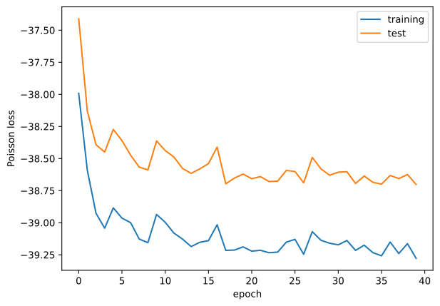
= torch.utils.data.DataLoader(= 64 , shuffle= True )= [], []for epoch in range (40 ):1 for xb, yb in loader:2 eval ()with torch.no_grad():float (poisson_loss(model(Xtr_t), ytr_t)))float (poisson_loss(model(Xte_t), yte_t)))print (f"final training loss: { train_curve[- 1 ]:.4f} " )print (f"final test loss: { test_curve[- 1 ]:.4f} " )
1
Training mode. Dropout is active and batch norm uses the batch statistics.
2
Evaluation mode. Dropout is off and batch norm uses the running statistics. Forgetting this is a common bug, and it makes the model look worse than it is.
final training loss: -39.2285
final test loss:     -38.6720
= plt.subplots()= "training" )= "test" )set (xlabel= "epoch" , ylabel= "Poisson loss" )
Comparing to the GLM
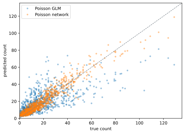
from sklearn.linear_model import PoissonRegressorfrom sklearn.metrics import mean_poisson_deviance= PoissonRegressor(alpha= 1e-4 , max_iter= 5000 ).fit(sc.transform(Xtr), ytr)eval ()with torch.no_grad():= model(Xte_t).numpy()= glm.predict(sc.transform(Xte))print (f"Poisson GLM deviance: { mean_poisson_deviance(yte, glm_pred):.4f} " )print (f"Poisson network deviance: { mean_poisson_deviance(yte, net_pred):.4f} " )
Poisson GLM deviance:     5.4424
Poisson network deviance: 1.2080
= plt.subplots()"." , alpha= 0.35 , label= "Poisson GLM" )"." , alpha= 0.35 , label= "Poisson network" )= [0 , yte.max () * 1.05 ]= "--" , lw= 1 , color= "#7a838b" )set (xlabel= "true count" , ylabel= "predicted count" , xlim= lim, ylim= lim)
If the network does not beat the GLM with good features, we keep the GLM. It is faster, it is easier to explain, and it has fewer ways to go wrong.
Reading the residuals
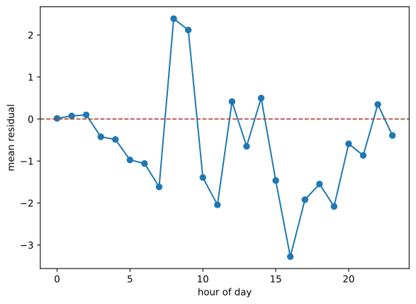
= np.round (np.arctan2(Xte[:, 0 ], Xte[:, 1 ]) * 24 / (2 * np.pi)) % 24 = yte - net_pred= plt.subplots()= pd.Series(resid).groupby(hour_te).mean()"o-" )0 , color= "#a8452f" , lw= 1.2 , ls= "--" )set (xlabel= "hour of day" , ylabel= "mean residual" )
A pattern left in the residuals is a predictor we have not used yet, not randomness. This plot is worth making for every predictor.
Where it goes wrong
Four mistakes come back every year.
Standardizing before the split. The test mean leaks into the training set. Fit the scaler on the training part only.
Using squared error on counts. It fits the busy hours and ignores the quiet ones, and it predicts negative rentals at night.
Tuning against the test set. After the third look it is a validation set, and the number you report is optimistic.
Forgetting model.eval(). Dropout stays on and the predictions are noisy.