Random forests and boosting

Examples

A single tree has high variance. Averaging reduces variance, so we average many trees.

Bagging

If we had \(B\) independent training sets we could fit \(B\) trees and average their predictions. The variance of the average would be \(B\) times smaller.

We only have one training set, so we resample from it with replacement. Each resample gives a slightly different tree. This is called bagging, from bootstrap aggregating.

Random forests

Bagged trees are still correlated. If one predictor is much stronger than the others, almost every tree splits on it first, and the trees end up similar.

A random forest adds a second source of randomness. At every split it considers only a random subset of the predictors, usually \(\sqrt{p}\) of them for classification. This forces the trees apart and the average improves.

import numpy as np
import matplotlib.pyplot as plt
from sklearn.ensemble import RandomForestRegressor, GradientBoostingRegressor
from sklearn.tree import DecisionTreeRegressor

rng = np.random.default_rng(10)

def f(x):
    return np.sin(2 * x) + 2 * (x - 0.5) ** 3 - 0.5 * x

x = rng.uniform(0, 1, 120)
y = f(x) + rng.normal(0, 0.15, 120)
X = x.reshape(-1, 1)
grid = np.linspace(0, 1, 500).reshape(-1, 1)

one = DecisionTreeRegressor(max_depth=6).fit(X, y)
forest = RandomForestRegressor(n_estimators=300, random_state=0).fit(X, y)

fig, ax = plt.subplots()
ax.plot(x, y, "o", alpha=0.4, label="data")
ax.plot(grid, f(grid[:, 0]), color="#7a838b", ls="--", lw=1.4, label="truth")
ax.plot(grid, one.predict(grid), label="one tree")
ax.plot(grid, forest.predict(grid), label="random forest")
ax.set(xlabel="x", ylabel="y")
ax.legend()
plt.show()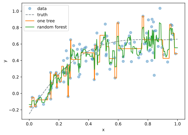

Figure 50.1: One tree against a forest of 300 trees. The forest is smoother, because it is an average of many step functions with different steps.

Note that a forest does not overfit as we add trees. More trees only reduce variance. The depth of the trees is what controls flexibility.

Gradient boosting

Boosting is the other way round. Instead of averaging many strong trees fitted independently, it adds many weak trees fitted in sequence, each one on the residuals of what came before.

\[ \hat f \leftarrow \hat f + \nu \, \hat t \]

where \(\hat t\) is a small tree fitted to the residuals and \(\nu\) is the learning rate, usually 0.01 to 0.1.

Boosting can overfit if we add too many trees. The number of trees is a hyper-parameter here, unlike in a forest.

fig, ax = plt.subplots()
ax.plot(x, y, "o", alpha=0.4, label="data")
ax.plot(grid, f(grid[:, 0]), color="#7a838b", ls="--", lw=1.4, label="truth")
for n_est in [5, 50, 2000]:
    b = GradientBoostingRegressor(n_estimators=n_est, learning_rate=0.1,
                                  max_depth=3, random_state=0).fit(X, y)
    ax.plot(grid, b.predict(grid), label=f"{n_est} trees")
ax.set(xlabel="x", ylabel="y")
ax.legend()
plt.show()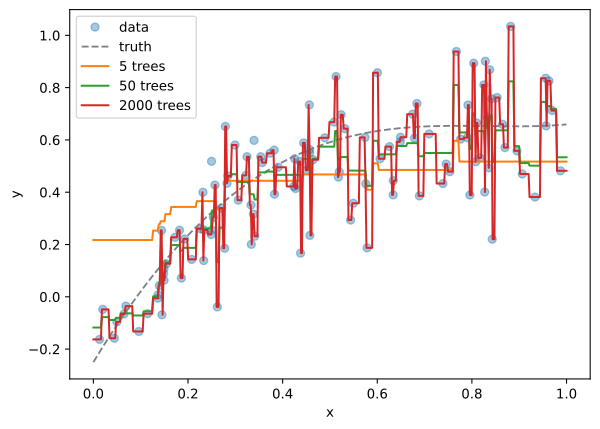

Figure 50.2: Gradient boosting with three numbers of trees. Too many trees start fitting the noise.

Which one

A random forest has few hyper-parameters and its defaults usually work. It is the right first thing to try on tabular data.

Gradient boosting is usually a little better if it is tuned, and a lot worse if it is not. The three parameters that matter are the number of trees, the learning rate and the depth. They interact, so tune them together.

For serious work use xgboost, lightgbm or catboost, which are faster and handle categorical predictors better than sklearn.

Variable importance

p = 8
Xp = rng.normal(0, 1, (600, p))
yp = 3 * Xp[:, 0] - 2 * Xp[:, 1] + 1.5 * Xp[:, 2] * Xp[:, 0] + rng.normal(0, 1, 600)

rf = RandomForestRegressor(n_estimators=300, random_state=0).fit(Xp, yp)
imp = rf.feature_importances_ / rf.feature_importances_.max()

fig, ax = plt.subplots(figsize=(5.4, 2.8))
ax.barh(np.arange(p), imp, color="#a8c8d6")
ax.set(yticks=np.arange(p), yticklabels=[f"x{i+1}" for i in range(p)],
       xlabel="relative importance")
plt.show()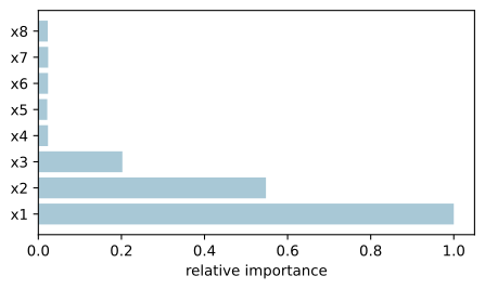

Figure 50.3: Variable importance in a random forest. Only three of the eight predictors carry signal.

The importance of a predictor is how much the loss dropped, over all splits on that predictor, over all trees. It is usually reported relative to the largest.

This is worth comparing to the two other ways we have seen of asking which predictor matters. A regression coefficient is the effect of one predictor with the others held fixed. The lasso sets irrelevant coefficients to zero. Variable importance needs no linear model, so it also picks up predictors that only matter in interaction with others, like \(x_3\) above.

None of the three is a causal statement.