Mixtures and density

Examples

k-means assigns every point to exactly one cluster and treats all clusters as round and equally sized. Two other methods relax these assumptions in different ways.

Gaussian mixture models

A Gaussian mixture says that \(P(X)\) is a weighted sum of normal distributions,

\[ p(x) = \sum_{j=1}^{k} \pi_j \, \mathcal{N}(x; \mu_j, \Sigma_j), \qquad \sum_j \pi_j = 1 . \]

This is a model of the data generating process, not just an algorithm. We can therefore fit it by maximum likelihood, exactly as in week 2.

Two things follow. Each cluster has its own covariance matrix, so it can be elongated and tilted. And each point gets a probability of belonging to each cluster, instead of a hard assignment.

import numpy as np
import matplotlib.pyplot as plt
from sklearn.cluster import KMeans, DBSCAN
from sklearn.mixture import GaussianMixture

rng = np.random.default_rng(11)

means = [[0, 0], [5, 5], [-5, 5]]
covs = [[[1, 0.8], [0.8, 1]], [[1, -0.6], [-0.6, 1]], [[1, 0], [0, 1]]]
X = np.vstack([rng.multivariate_normal(m, c, 150) for m, c in zip(means, covs)])

gmm = GaussianMixture(n_components=3, random_state=0).fit(X)
proba = gmm.predict_proba(X)
lab = proba.argmax(axis=1)
conf = proba.max(axis=1)

fig, ax = plt.subplots(figsize=(4.6, 4.2))
for j in range(3):
    sel = lab == j
    ax.scatter(X[sel, 0], X[sel, 1], s=14, alpha=conf[sel] ** 3)
ax.set(xticks=[], yticks=[])
plt.show()

1

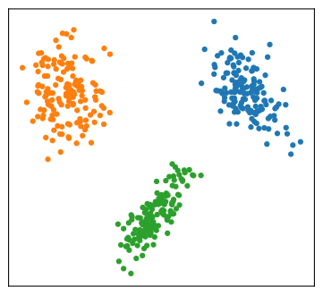
Points near a boundary are almost transparent. Those are the points where the model is unsure.

Figure 57.1: A Gaussian mixture with three components. The colour is the most likely cluster and the transparency is the confidence.

print("points with confidence below 0.9:", int((conf < 0.9).sum()))
print("smallest confidence:", round(float(conf.min()), 3))

points with confidence below 0.9: 0
smallest confidence: 0.999

This is the main advantage over k-means. A point can be reported as uncertain instead of being forced into a cluster.

cov = [[4.0, 3.4], [3.4, 4.0]]
A = rng.multivariate_normal([0, 0], cov, 200)
B = rng.multivariate_normal([4, -3], cov, 200)
E = np.vstack([A, B])

fig, axes = plt.subplots(1, 2, figsize=(6.6, 3.2))
for ax, (name, lab) in zip(axes, [
        ("k-means", KMeans(n_clusters=2, n_init=10, random_state=0).fit_predict(E)),
        ("Gaussian mixture", GaussianMixture(n_components=2, random_state=0).fit_predict(E))]):
    for j in np.unique(lab):
        ax.plot(E[lab == j, 0], E[lab == j, 1], "o", ms=3)
    ax.set_title(name, fontsize=9)
    ax.set(xticks=[], yticks=[])
plt.show()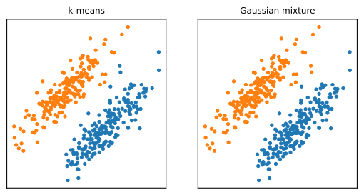

Figure 57.2: Elongated clusters. k-means cuts them because it assumes round shapes. The mixture fits the shapes.

Note that k-means is a special case of a Gaussian mixture. Fix all covariances to \(\sigma^2 I\), let \(\sigma \to 0\), and the soft assignments become hard ones.

DBSCAN

DBSCAN takes a different view. A cluster is a region where points are dense, and the rest is noise.

It has two parameters. The radius \(\varepsilon\) and the minimum number of points min_samples. A point is a core point if at least min_samples points lie within \(\varepsilon\) of it. Core points that are within \(\varepsilon\) of each other belong to the same cluster. Points that are near a core point join its cluster. Everything else is labelled noise.

Two things follow. The number of clusters is not given in advance, it comes out of the density. And points can be assigned to no cluster at all, which none of the other methods allow.

t = rng.uniform(0, np.pi, 200)
moons = np.vstack([
    np.column_stack([np.cos(t), np.sin(t)]) + rng.normal(0, 0.07, (200, 2)),
    np.column_stack([1 - np.cos(t), 0.5 - np.sin(t)]) + rng.normal(0, 0.07, (200, 2))])

for eps in [0.1, 0.22, 0.6]:
    lab = DBSCAN(eps=eps, min_samples=5).fit_predict(moons)
    n_clusters = len(set(lab)) - (1 if -1 in lab else 0)
    print(f"eps = {eps:4}   clusters = {n_clusters}   noise = {(lab == -1).sum()}")

1

Two interleaving half circles. No straight cut separates them, which is the point of the example.

eps =  0.1   clusters = 6   noise = 37
eps = 0.22   clusters = 2   noise = 0
eps =  0.6   clusters = 1   noise = 0

DBSCAN is sensitive to \(\varepsilon\). Too small and everything is noise. Too large and everything is one cluster.

The radius and the minimum count decide everything. On the moons there is a window of ε where it finds exactly two clusters. On data with no structure it labels almost everything noise, which is the honest answer.

And because it uses one global radius, it struggles when different clusters have very different densities.

Which method

	assumes	number of clusters	outliers
k-means	round, similar size	given	forced into a cluster
Gaussian mixture	elliptical	given	soft assignment
hierarchical	depends on linkage	chosen from the tree	forced into a cluster
DBSCAN	dense regions	comes out	labelled as noise

None of them is right in general. Run more than one, and be suspicious if they disagree.