Hierarchical clustering

Examples

Hierarchical clustering does not need the number of clusters in advance. It builds a whole tree of clusterings, and we cut it where we like.

The algorithm

1. Start with every point in its own cluster.
2. Repeat until one cluster is left.
   1. Find the two closest clusters.
   2. Merge them, and record the height at which they merged.

The result is a dendrogram. Cutting it at a given height gives a clustering.

Linkage

We need a distance between two sets of points, not between two points. That choice is called the linkage.

linkage	definition
single	\(\min_{x \in C_i, y \in C_j} d(x, y)\)
complete	\(\max_{x \in C_i, y \in C_j} d(x, y)\)
average	the mean over all pairs
Ward	the merge that increases the within-cluster sum of squares the least

An example

import numpy as np
import matplotlib.pyplot as plt
from scipy.cluster.hierarchy import dendrogram, linkage, fcluster

rng = np.random.default_rng(11)

centres = np.array([[0., 0.], [4., 4.], [-4., 4.]])
X = np.vstack([rng.normal(c, 1.0, (25, 2)) for c in centres])

Z = linkage(X, method="complete")

fig, ax = plt.subplots(figsize=(6.6, 3.0))
dendrogram(Z, ax=ax, no_labels=True, color_threshold=6.5,
           above_threshold_color="#7a838b")
ax.axhline(6.5, color="#a8452f", lw=1.2, ls="--")
ax.set(ylabel="merge height")
plt.show()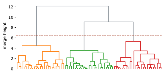

Figure 56.1: The dendrogram with complete linkage. The horizontal line is a cut that gives three clusters.

The height of a merge is the distance between the two clusters at that moment. A long vertical line means the two clusters were far apart, which is a sign of real structure. Many short merges near the bottom mean the points are all similar.

Move the cut and watch the clusters appear below. Change the linkage and note that single linkage merges at much lower heights, which is the chaining effect.

labels = fcluster(Z, t=3, criterion="maxclust")
print("cluster sizes:", np.bincount(labels)[1:])

cluster sizes: [25 25 25]

The linkage matters

fig, axes = plt.subplots(1, 4, figsize=(6.8, 2.0))
for ax, method in zip(axes, ["single", "complete", "average", "ward"]):
    lab = fcluster(linkage(X, method=method), t=3, criterion="maxclust")
    for j in np.unique(lab):
        ax.plot(X[lab == j, 0], X[lab == j, 1], "o", ms=2.5)
    ax.set_title(method, fontsize=9)
    ax.set(xticks=[], yticks=[])
plt.show()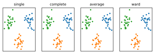

Figure 56.2: The same data cut into three clusters with four linkages.

Single linkage tends to produce one large cluster and several tiny ones, because a single close pair is enough to merge two groups. This is called chaining.

Complete and average linkage produce more balanced clusters. Ward tends to produce clusters of similar size, which is a good default and also an assumption we may not want.

When single linkage wins

Chaining is not always bad. If the clusters are long and thin, single linkage is the only one of the four that finds them.

t = rng.uniform(0, np.pi, 120)
moon1 = np.column_stack([np.cos(t), np.sin(t)]) + rng.normal(0, 0.06, (120, 2))
moon2 = np.column_stack([1 - np.cos(t), 0.5 - np.sin(t)]) + rng.normal(0, 0.06, (120, 2))
moons = np.vstack([moon1, moon2])

fig, axes = plt.subplots(1, 2, figsize=(6.6, 2.9))
for ax, method in zip(axes, ["single", "complete"]):
    lab = fcluster(linkage(moons, method=method), t=2, criterion="maxclust")
    for j in np.unique(lab):
        ax.plot(moons[lab == j, 0], moons[lab == j, 1], "o", ms=3)
    ax.set_title(method, fontsize=9)
    ax.set(xticks=[], yticks=[])
plt.show()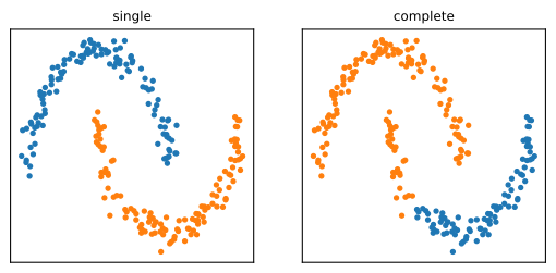

Figure 56.3: Two moons. Single linkage follows the shape, complete linkage cuts across it.

Small decisions with big consequences

Before we can cluster anything we have made several choices. The distance measure. Whether to standardize. The linkage. Where to cut.

None of these is given by the data, and all of them change the answer. Report them, and check whether the conclusion survives a different choice.