k-means

Examples

The algorithm

Place \(k\) centroids.
Repeat until nothing changes.
1. Assign each point to the nearest centroid.
2. Move each centroid to the mean of the points assigned to it.

The objective is the within-cluster sum of squares,

\[ W_k = \min_{C_1, \dots, C_k} \sum_{j=1}^{k} \sum_{i \in C_j} \|x_i - \mu_j\|^2 , \qquad \mu_j = \frac{1}{|C_j|}\sum_{i \in C_j} x_i . \]

This is what sklearn reports as inertia_.

Each step of the algorithm lowers \(W_k\) or leaves it unchanged, so it converges. It converges to a local minimum, not the global one.

An example

import numpy as np
import matplotlib.pyplot as plt
from sklearn.cluster import KMeans

rng = np.random.default_rng(11)

centres = np.array([[0., 0.], [4., 4.], [-4., 4.]])
X = np.vstack([rng.normal(c, 1.0, (120, 2)) for c in centres])

Step through the iterations. At iteration 0 the centroids are placed and nothing is assigned yet. Each step assigns every point to the nearest centroid, then moves each centroid to the mean of its points. Change the initialization to see it converge somewhere else.

It depends on where we start

This is why sklearn runs the algorithm several times by default and keeps the best. That is the n_init argument. Do not set it to 1 unless you know why.

Clusters can become empty

If no point is closest to a centroid, that cluster is empty and its mean is undefined. Implementations handle this by moving the centroid somewhere else, but it means we may end up with fewer than \(k\) clusters.

k-means assumes round clusters of similar size

Four methods on four data sets. Only DBSCAN can label a point as noise, and only DBSCAN decides the number of clusters for itself. On data with no structure, all four still return clusters.

The moons are separated by a straight cut through the middle. The small dense cluster is swallowed by the large one.

How many clusters

The silhouette score measures, for each point, how much closer it is to its own cluster than to the nearest other cluster. For point \(i\),

\[ s_i = \frac{b_i - a_i}{\max(a_i, b_i)}, \]

where \(a_i\) is the mean distance to the points of its own cluster and \(b_i\) is the mean distance to the points of the nearest other cluster. It lies between \(-1\) and \(1\). We average over all points and pick the \(k\) with the highest value.

from sklearn.metrics import silhouette_score

ks = range(2, 9)
inertia = [KMeans(n_clusters=k, n_init=10, random_state=0).fit(X).inertia_ for k in ks]
sil = [silhouette_score(X, KMeans(n_clusters=k, n_init=10, random_state=0).fit_predict(X))
       for k in ks]

fig, axes = plt.subplots(1, 2, figsize=(6.6, 2.8))
axes[0].plot(list(ks), inertia, "o-")
axes[0].set(xlabel="k", ylabel="$W_k$")
axes[1].plot(list(ks), sil, "o-")
axes[1].set(xlabel="k", ylabel="silhouette")
plt.show()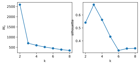

Figure 55.1: The objective and the silhouette score against k. The objective falls forever. The silhouette has a maximum at the right answer.

Note that \(W_k\) keeps falling as \(k\) grows. This is also why cross-validation on \(W_k\) does not work. With more centroids, any held-out point is closer to some centroid.

The gap statistic is the other common approach. It compares \(\log W_k\) to the value obtained on uniformly random data, and picks the smallest \(k\) at which the gap stops growing.

Silhouette and gap statistic often disagree. If the answer depends strongly on the method, that is information. The data probably has no clear cluster structure.

k-means on the iris measurements, with the true species shown below for comparison. At two clusters the two similar species merge. At three the split is close to the species but not the same, and no choice of k recovers them exactly.

On MNIST

import numpy as np
from sklearn.cluster import KMeans
from sklearn.datasets import fetch_openml

mnist = fetch_openml("mnist_784", version=1, as_frame=True, parser="auto")
X = mnist.data.values[:10000] / 255.0
digits = mnist.target.values[:10000].astype(int)

km = KMeans(n_clusters=10, n_init=5, random_state=0).fit(X)
print("cluster sizes:", np.bincount(km.labels_))

1: Ten thousand of the seventy thousand, so that this page builds quickly.

cluster sizes: [ 529  754 1053 1486  468  935 1476 1412  736 1151]

import matplotlib.pyplot as plt

fig, axes = plt.subplots(1, 10, figsize=(6.6, 0.9))
for j, ax in enumerate(axes):
    ax.imshow(km.cluster_centers_[j].reshape(28, 28), cmap="gray")
    ax.set(xticks=[], yticks=[])
    ax.set_title(str(np.bincount(digits[km.labels_ == j]).argmax()), fontsize=8)
plt.show()

Figure 55.2: The ten centroids. Each one is the average of the images in its cluster, so it looks like a blurred digit.

The number above each centroid is the digit that is most common in that cluster. Nobody gave the algorithm the labels.

import pandas as pd

tab = pd.crosstab(km.labels_, digits)
tab.index.name, tab.columns.name = "cluster", "digit"
tab

digit	0	1	2	3	4	5	6	7	8	9
cluster
0	471	0	10	14	0	19	8	2	3	2
1	0	579	56	6	27	5	5	41	27	8
2	34	2	24	224	1	220	13	1	530	4
3	2	2	5	14	342	35	0	621	33	432
4	425	0	1	1	1	10	12	4	7	7
5	27	0	28	9	14	19	816	1	18	3
6	6	540	125	105	64	262	134	89	90	61
7	5	1	18	21	520	59	12	306	26	444
8	2	2	663	30	11	1	10	4	11	2
9	29	1	61	608	0	233	4	1	199	15

Some clusters contain almost only one digit. Others mix a few, and the same digit can be split across two clusters, because it is written in two different ways. This is not a failure. It tells us which digits look alike in pixel space.