Beyond PCA

Examples

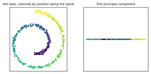
PCA is a linear method. It finds a linear subspace. If the data lies on a curved surface, a linear subspace is the wrong description.

Where PCA fails

import numpy as np
import matplotlib.pyplot as plt
from sklearn.decomposition import PCA

rng = np.random.default_rng(12)

t = rng.uniform(1.5 * np.pi, 4.5 * np.pi, 600)
X = np.column_stack([t * np.cos(t), t * np.sin(t)]) + rng.normal(0, 0.3, (600, 2))

Z = PCA(n_components=1).fit_transform(X)

fig, axes = plt.subplots(1, 2, figsize=(6.6, 3.0))
axes[0].scatter(X[:, 0], X[:, 1], c=t, s=5, cmap="viridis")
axes[0].set_title("the data, coloured by position along the spiral", fontsize=8)
axes[0].set_aspect("equal")
axes[1].scatter(Z[:, 0], np.zeros_like(Z[:, 0]), c=t, s=5, cmap="viridis")
axes[1].set_title("first principal component", fontsize=8)
for ax in axes:
    ax.set(xticks=[], yticks=[])
plt.show()

Figure 62.1: Points on a spiral. PCA cannot unroll it, because unrolling is not a linear map.

The colours are shuffled on the right. Points that are far apart on the spiral land on top of each other. The intrinsic dimension of this data is one, but the one dimension is not a straight line.

t-SNE

t-SNE builds a low dimensional map in which points that are close in the original space stay close.

It works with probabilities. For each pair of points it defines a probability that one would pick the other as a neighbour, in the original space and in the map. It then moves the map points until the two sets of probabilities agree, in the sense of the Kullback-Leibler divergence.

The main parameter is the perplexity, which is roughly how many neighbours each point pays attention to. Values between 5 and 50 are usual.

PCA against t-SNE at three perplexities, on a spiral and on the digits. On the spiral the colours run along the curve. PCA shuffles them, t-SNE keeps them together.

The ten digits separate much more clearly than they do in the first two principal components.

Three warnings.

The distance between two clusters in a t-SNE plot means nothing. Only local neighbourhoods are preserved.

The size of a cluster means nothing either. t-SNE expands sparse regions and compresses dense ones.

Different random seeds give different pictures. Run it more than once before drawing a conclusion.

UMAP

UMAP does something similar with a different construction, based on a graph of nearest neighbours. In practice it is faster than t-SNE, it scales to larger data sets, and it preserves more of the global structure.

import umap

reducer = umap.UMAP(n_neighbors=15, min_dist=0.1, random_state=0)
E = reducer.fit_transform(D)

The parameter n_neighbors plays a similar role to the perplexity. min_dist controls how tightly points are allowed to pack together.

The same warnings apply. These are tools for looking at data, not for measuring it. Do not compute distances on a t-SNE or UMAP embedding and treat them as meaningful.

Matrix completion

A different use of the same idea. Suppose the matrix \(X\) has missing entries, for example ratings of films by users, where nobody has seen every film.

If we assume the full matrix has low rank, we can fill in the gaps. We look for a rank \(L\) matrix that agrees with the entries we do observe, and read the missing entries off it.

This is how recommender systems started. The low rank assumption says there are a few underlying factors, and every user and every film is described by its position on those factors.

Comparing the methods

	finds	preserves	use for
PCA	a linear subspace	global variance	preprocessing, compression, denoising
t-SNE	a non-linear map	local neighbourhoods	looking at clusters
UMAP	a non-linear map	local, some global	the same, on larger data

PCA is the one to use when the output feeds into another model, because it is a linear map that can be applied to new points. t-SNE cannot be applied to a new point at all without refitting.