Compression, denoising and regression

Examples

Once we can move between the original coordinates and the scores, several things become possible.

Compression

Keeping \(L\) components and reconstructing gives a lossy approximation. We store \(n \times L\) scores and \(p \times L\) loadings instead of \(n \times p\) numbers.

import numpy as np
import matplotlib.pyplot as plt
from sklearn.datasets import load_digits
from sklearn.decomposition import PCA

rng = np.random.default_rng(12)

digits = load_digits()
X = digits.images.reshape(-1, 64)

The number of components kept, against the reconstruction of eight digits and the scree plot. Switch to the noisy data and find the number of components at which the reconstruction is closest to the clean image.

With 8 of 64 components we keep most of what a person needs to read the digit, and store a fraction of the numbers.

Three dimensional data that really lies close to a plane. With one component the reconstruction collapses onto a line, with two it lands on the plane, with three it is exact.

Denoising

If the signal lies in a low dimensional subspace and the noise is spread over all directions, then projecting onto the first few components removes more noise than signal.

Xn = X + rng.normal(0, 4.0, X.shape)

p = PCA(n_components=12).fit(Xn)
Xd = p.inverse_transform(p.transform(Xn))

fig, axes = plt.subplots(3, 8, figsize=(6.6, 2.7))
for col in range(8):
    axes[0, col].imshow(X[col].reshape(8, 8), cmap="gray")
    axes[1, col].imshow(Xn[col].reshape(8, 8), cmap="gray")
    axes[2, col].imshow(Xd[col].reshape(8, 8), cmap="gray")
    for row in range(3):
        axes[row, col].set(xticks=[], yticks=[])
for row, name in enumerate(["clean", "noisy", "denoised"]):
    axes[row, 0].set_ylabel(name, fontsize=8)
plt.show()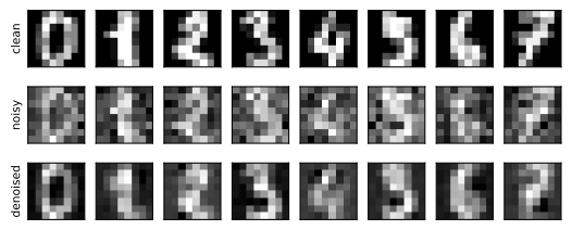

Figure 61.1: Noisy digits and their reconstruction from 12 components.

print("error before denoising:", round(float(np.mean((Xn - X) ** 2)), 2))
print("error after denoising: ", round(float(np.mean((Xd - X) ** 2)), 2))

error before denoising: 15.98
error after denoising:  7.28

Note the assumption. This only works if the signal really is low dimensional. If it is not, we remove signal along with the noise.

Recovering a generative model

If the data was generated from a few hidden factors and a linear map, PCA can find the subspace those factors span.

k, p_dim, n = 3, 30, 500
A = rng.normal(0, 1, (p_dim, k))
H = rng.normal(0, 1, (n, k))
D = H @ A.T + rng.normal(0, 0.5, (n, p_dim))

pd_ = PCA().fit(D)

fig, ax = plt.subplots(figsize=(5.0, 2.6))
ax.plot(np.arange(1, p_dim + 1), pd_.explained_variance_ratio_, "o-")
ax.set(xlabel="component", ylabel="proportion of variance")
plt.show()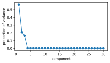

Figure 61.2: Three hidden factors mapped into 30 dimensions with noise. The scree plot shows three components.

PCA does not recover the factors themselves. Any rotation of the three factors generates the same data, so the individual components are not identifiable. What PCA recovers is the subspace they span.

Principal component regression

If \(p\) is large and the predictors are correlated, we can run PCA first and regress on the first \(L\) scores.

from sklearn.linear_model import LinearRegression, Ridge
from sklearn.model_selection import KFold, cross_val_score
from sklearn.pipeline import make_pipeline
from sklearn.preprocessing import StandardScaler

beta = np.zeros(p_dim)
beta[:5] = [2.0, -1.5, 1.0, 0.8, -0.6]
yv = D @ beta + rng.normal(0, 1.0, n)

cv = KFold(5, shuffle=True, random_state=0)


def rmse(model):
    s = cross_val_score(model, D, yv, cv=cv, scoring="neg_root_mean_squared_error")
    return -s.mean()


print("plain linear regression:", round(rmse(
    make_pipeline(StandardScaler(), LinearRegression())), 4))
for L in [2, 3, 5, 10]:
    m = make_pipeline(StandardScaler(), PCA(n_components=L), LinearRegression())
    print(f"PCR with L = {L:2d}:          {rmse(m):.4f}")
print("ridge:                  ", round(rmse(
    make_pipeline(StandardScaler(), Ridge(alpha=10.0))), 4))

plain linear regression: 1.0106
PCR with L =  2:          2.3827
PCR with L =  3:          1.7930
PCR with L =  5:          1.8012
PCR with L = 10:          1.3533
ridge:                   1.0674

The number of components \(L\) is a hyper-parameter, chosen by cross-validation like any other.

Principal component regression is closely related to ridge regression. Both shrink the directions in which the data varies little. PCR does it abruptly, by dropping them completely. Ridge does it gradually, shrinking each direction by a factor that depends on its variance.

There is an important caveat. PCA looks only at \(X\) and never at \(y\). The directions of largest variance in \(X\) need not be the directions that predict \(y\). If the response depends on a low variance direction, PCR will throw it away. Partial least squares is the method that fixes this by using \(y\) as well.