Both models on this page fit a Bernoulli distribution by maximum likelihood. They differ in one line: what computes \(\eta\).
More than one predictor
With \(p\) predictors the fitted probability is a surface over the input space, and the set of points where it crosses the threshold is the decision boundary. For a linear \(\eta\) that boundary is \(\beta_0 + \beta_1x_1 + \cdots + \beta_px_p = 0\), a hyperplane, whatever the threshold happens to be.
With two predictors the probability is a surface and the decision boundary is a line. Move the threshold and watch the boundary shift without the probability changing at all.
Moving the threshold slides the boundary. It never bends it. That is a property of the function family, not of the data, and it is the thing a network changes.
The same data, twice
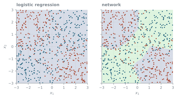
We generate a problem no straight line can solve: the two classes sit in alternating quadrants, softened by noise.
import numpy as npimport pandas as pdimport torchimport matplotlib.pyplot as plttorch.manual_seed(7)rng = np.random.default_rng(7)def make(n, rng): X = rng.uniform(-3, 3, (n, 2)) eta =1.4* X[:, 0] * X[:, 1] y = (rng.random(n) <1/ (1+ np.exp(-eta))).astype(np.float32)return X.astype(np.float32), yXtr, ytr = make(600, rng)Xte, yte = make(4000, rng)print("class balance:", round(float(ytr.mean()), 3))
1
The product of the two inputs. A linear function of \(x_1\) and \(x_2\) cannot reproduce it, which is the point.
One output, and no activation on it. The raw number is\(\eta\).
2
The Bernoulli row of the table. BCEWithLogitsLoss applies \(s(\cdot)\) and takes the negative log-likelihood in one step, which is numerically safer than computing the probability first and then its logarithm.
training accuracy: 0.83
test accuracy:     0.842
The identical network with torch.nn.Linear(32, 1) and torch.nn.MSELoss() would be the week 6 regression model. One line of the network changed, and it is the loss.
Figure 38.1: The decision boundary of each model at the threshold 0.5, over the training data. The linear model has one straight line to work with.
The same likelihood with a widening hidden layer. At zero hidden neurons this is logistic regression and the boundary is a straight line, whatever the data does. Two neurons are already enough to carve the plane into quadrants; the rest buys parameters and a little overfitting. Change the training set and watch how much the wide models move and how little the linear one does.
When the gain is small
The previous example was built so that a network would win, and it won by more than thirty points. That is not the usual size of the effect. Here is a problem where the same substitution buys almost nothing.
The spam data is text, represented as in week 4 by word frequencies, this time with every word of the training emails in the lexicon.
Bag of words. Each column counts how often one word occurs in one email.
2
Divided by the length of the email, so that a long email does not dominate.
3
transform, not fit_transform. The vocabulary has to be the one the model was trained on, or the columns would mean different things.
emails: 2000 vocabulary: 28128
Each word is one predictor, so \(p\) is in the tens of thousands while \(n\) is 2000. With \(p > n\) the training data can be fitted perfectly, and it will be. This is why week 3 was about regularization.
MLPClassifier is sklearn’s shortcut for a network with a softmax output and the cross-entropy loss. Fewer options than torch, which for a problem this size is an advantage.
model
training accuracy
test accuracy
0
logistic regression
0.996
0.968
1
network
1.000
0.987
The network is ahead, by about two points rather than thirty. Count what it cost: the linear model has one parameter per word plus an intercept, about 28000 of them, and the network has one per word per hidden unit, about 1.8 million. The signal in this representation really is close to additive in the word frequencies, so most of that flexibility has nothing to do.
Notice also that both models fit the training set essentially perfectly. Neither is penalized here, and with \(p \gg n\) that is exactly what week 3 warned about. A ridge penalty on the linear model is a far cheaper way to spend effort on this problem than a hidden layer, and it is a good exercise to check how much of the two-point gap survives it.
words = np.array(vectorizer.get_feature_names_out())order = np.argsort(spam_lin.coef_[0])pd.DataFrame({"most ham-like": words[order[:10]],"most spam-like": words[order[-10:]][::-1]})
most ham-like
most spam-like
0
schedul
your
1
enron
http
2
hourahead
more
3
louis
click
4
start
www
5
hour
here
6
messag
you
7
date
remov
8
if
onlin
9
origin
net
And this is the other thing the linear model gives you, for free and with no extra machinery. There is no equivalent table for the network: its first layer mixes all 28000 words before anything interpretable happens. Whether that matters is a question about what the model is for.
Not every word needs a column. A lexicon of the words that are neither very rare nor very frequent is much smaller.
from sklearn.model_selection import cross_val_scorefrom sklearn.pipeline import make_pipelinefrom sklearn.preprocessing import Normalizerlexicon_lin = make_pipeline( CountVectorizer(min_df=0.02, max_df=0.3), Normalizer(norm="l1"), LogisticRegression(penalty=None, max_iter=2000))lexicon_lin.fit(train["text"], y_train)print("words in the lexicon:", len(lexicon_lin[0].vocabulary_))print("test accuracy:", round(lexicon_lin.score(test["text"], y_test), 3))print("cross-validated on the training emails:",round(cross_val_score(lexicon_lin, train["text"], y_train, cv=5).mean(), 3))
1
Keep the words that occur in at least 2% and at most 30% of the training emails.
2
Divides every row by its sum, which turns the counts into frequencies, as above.
words in the lexicon: 1082
test accuracy: 0.962
cross-validated on the training emails: 0.965
With a twenty-sixth of the words the test accuracy is almost unchanged. The vectorizer is now a step of the pipeline, so in cross-validation every fold builds its lexicon from its own training emails, like the scaler in week 4. A lexicon built once from all the emails would let the held-out ones decide which columns exist.
The gap between training and test accuracy on both models is large. Which of the two is actually better, and how much of that gap is threshold artefact rather than model quality, is the next question but one.