Top left, the data and the fitted line. Top right, the level lines of the regularized loss, with the fit at its minimum. Bottom left, the two coefficients along the whole path. Bottom right, the level lines of the unregularized loss, the same path, and the constraint region \(\|\theta\|_2^2
\le s\) that this \(\lambda\) corresponds to. At \(\lambda = 0\) nothing is constrained, so the whole plane is allowed.
At \(\lambda_2 = 0\) the fit is \(\beta_0 = 0.074\), \(\beta_1 = 0.083\). Nothing happens until about \(\lambda_2 = 10^{-3}\); then both coefficients are pulled towards the origin, \(\beta_1\) faster. At \(\lambda_2 = 562\) they are 0.0002 and 0.0001 — small, but not zero. The two right hand plots are the same statement twice: the penalty moves the centre of the level lines, and the point where the path leaves the circle is where the unregularized loss is smallest among the parameters that penalty allows.
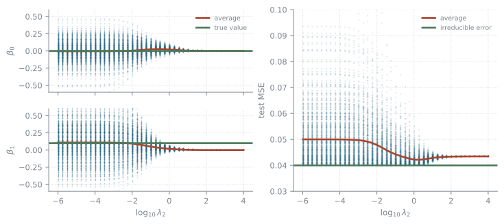
Regularization can decrease the variance, but it may increase the bias:
the simulation behind the figure
import numpy as npimport matplotlib.pyplot as pltlams = np.logspace(-6, 4, 41)loglam = np.log10(lams)sim = np.random.default_rng(12)test_x = sim.uniform(0, 1, 10**4) # one test set, used by every fittest_y =0.1* test_x +0.2* sim.standard_normal(10**4)mx, mxx = test_x.mean(), (test_x**2).mean()my, myy = test_y.mean(), (test_y**2).mean()mxy = (test_x * test_y).mean()def ridge_path(x, y): # all 41 penalties at once a, b, c, d = x.mean(), y.mean(), (x**2).mean(), (x * y).mean() b1 = (d - a * b / (1+ lams)) / (c - a**2/ (1+ lams) + lams)return (b - b1 * a) / (1+ lams), b1B0, B1 = np.empty((41, 500)), np.empty((41, 500))for k inrange(500): x = sim.uniform(0, 1, 10) B0[:, k], B1[:, k] = ridge_path(x, 0.1* x +0.2* sim.standard_normal(10))# the test error from the test set's moments: exact, and it turns 20 500# passes over 10 000 points into one array expressionmse = (B0**2+2* B0 * B1 * mx -2* B0 * my+ B1**2* mxx -2* B1 * mxy + myy)fig, ax = plt.subplot_mosaic([["b0", "mse"], ["b1", "mse"]], figsize=(8.8, 3.6))cloud =dict(s=1.5, alpha=0.25, color="#1f5f7a", linewidths=0, rasterized=True)xs = np.repeat(loglam, 500)for key, vals, truth in (("b0", B0, 0.0), ("b1", B1, 0.1)): ax[key].scatter(xs, vals.ravel(), **cloud) ax[key].plot(loglam, vals.mean(axis=1), lw=2, color="#a8452f", label="average") ax[key].axhline(truth, lw=2, color="#4c7a5a", label="true value") ax[key].set(ylabel=rf"$\beta_{key[-1]}$", ylim=(-0.6, 0.6))ax["b0"].tick_params(labelbottom=False)ax["b0"].legend(fontsize=7, loc="upper right")ax["b1"].set_xlabel(r"$\log_{10}\lambda_2$")ax["mse"].scatter(xs, mse.ravel(), **cloud)ax["mse"].plot(loglam, mse.mean(axis=1), lw=2, color="#a8452f", label="average")ax["mse"].axhline(0.2**2, lw=2, color="#4c7a5a", label="irreducible error")ax["mse"].set(xlabel=r"$\log_{10}\lambda_2$", ylabel="test MSE", ylim=(0.03, 0.1))ax["mse"].legend(fontsize=7)plt.show()
Figure 17.1: Each dot is one of 500 training sets of ten points, fitted at every penalty. Left, the two coefficients with their average and the value the generator used. Right, the test error of each fit with its average and the irreducible error.
Unpenalized, the estimate of \(\beta_1\) is unbiased but useless: its average over the 500 training sets is 0.109, right on the generator’s 0.1, but its standard deviation is 0.25 — two and a half times the quantity being estimated. The penalty collapses that scatter and drags the average off the truth with it. At the best penalty, \(\log_{10}\lambda_2 = 0.25\), the spread is down to 0.014 and the average is 0.012, and the test error is at its lowest: 0.042 against 0.050 unpenalized, for an irreducible error of 0.040. When the regularization gets stronger, the slope is too strongly biased towards 0, and this bias dominates the error.
Lasso (L1)
The same four plots for the L1 penalty. The constraint region is a diamond with corners on the axes.
The coefficients do not approach zero here, they arrive: \(\beta_1\) is exactly 0 from \(\lambda_1 = 0.018\) onwards and \(\beta_0\) from 0.178. The corners of the diamond sit on the axes, and a corner is where one coefficient is zero, which is why L1 selects predictors and L2 only shrinks them.
The same penalty applies to any model, polynomial regression included.
A polynomial of the chosen degree fitted to the regression data with an L2 penalty \(\lambda\) on its coefficients. The readout is the mean squared distance between the fit and the data generator over \([0, 1]\).
At degree 20 with \(\lambda = 0\) the reducible error is 11. At \(\lambda = 10^{-4}\) it is 0.0020, better than a degree 4 polynomial reaches at the same \(\lambda\) (0.0075). Raise \(\lambda\) further and the fit straightens out and underfits instead.
The penalty goes on the end of the same pipeline that built the powers.
import pandas as pdimport matplotlib.pyplot as pltfrom sklearn.linear_model import lasso_pathfrom sklearn.preprocessing import StandardScalerweather = pd.read_csv("https://go.epfl.ch/bio322-weather2015-2018.csv")X = weather.iloc[:-5].drop(columns=["LUZ_wind_peak", "time"])y = weather["LUZ_wind_peak"][5:].valuesalphas, coefs, _ = lasso_path(StandardScaler().fit_transform(X), y, alphas=np.logspace(1, -2, 60))# one row per predictor, one column per lambda, largest lambda first, so the# first non-zero entry of a row is where that predictor entersnonzero = coefs !=0entered = np.where(nonzero.any(axis=1), nonzero.argmax(axis=1), len(alphas))first5 = np.argsort(entered, kind="stable")[:5]fig, ax = plt.subplots(figsize=(8.8, 3.6))loglam = np.log10(alphas)ax.plot(loglam, coefs.T, lw=0.7, color="#b8bfc4", zorder=1)for rank, (j, colour) inenumerate(zip(first5, ["#1f5f7a", "#a8452f", "#8a6a18","#4c7a5a", "#6b5b8a"]), 1): ax.plot(loglam, coefs[j], lw=2, color=colour, zorder=2, label=f"{rank}. {X.columns[j]}")ax.axhline(0, lw=0.7, color="#7a838b")ax.set(xlabel=r"$\log_{10}\lambda$", ylabel="coefficient")ax.legend(loc="upper left", fontsize=7.5, ncol=2, framealpha=0.9)ax.set_ylim(-5, 5)plt.show()for rank, j inenumerate(first5, 1):print(f"{rank}. {X.columns[j]:22s} enters at lambda = {alphas[entered[j]]:.2f}")print(f"{(entered ==len(alphas)).sum()} of {len(X.columns)} never leave zero")
1
The penalty treats every coefficient the same, but the predictors are not: one measured in metres gets a coefficient a thousand times smaller than the same predictor in millimetres, so the penalty hits it a thousand times less. Standardize before regularizing.
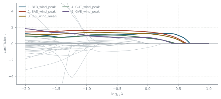
The lasso path for the wind peak in Luzern five hours ahead, over all 55 predictors. The five that leave zero first are drawn in colour and named; the other 50 are grey.
1. BER_wind_peak          enters at lambda = 4.41
2. BAS_wind_peak          enters at lambda = 3.92
3. LUZ_wind_mean          enters at lambda = 3.92
4. GUT_wind_peak          enters at lambda = 2.76
5. GVE_wind_peak          enters at lambda = 2.45
6 of 55 never leave zero
Read it from the right. At \(\lambda = 10\) the penalty is stronger than any predictor is worth and every coefficient is zero. Moving left weakens it, and the predictors leave zero one at a time; the height of a line is the coefficient that predictor would have in the model fitted at that \(\lambda\).
The order they leave in is a ranking, but a ranking given what is already in, not of each predictor on its own. The wind peak in Bern comes first, then Basel and Luzern’s own mean wind together, then Güttingen and Geneva — upwind gusts and the wind already blowing. The first pressure reading waits until \(\lambda \approx 1.5\), and a handful of predictors never enter at all. That is what makes the path worth drawing: one run gives the whole family of models from empty to full, it says how many predictors are actually earning their place, and a predictor that only repeats one already in the model stays flat at zero instead of splitting a coefficient with it.