There is no need to write networks by hand. In torch a network with a three-dimensional input, 30 hidden relu neurons and a two-dimensional output is
import numpy as npimport torchimport matplotlib.pyplot as plttorch.manual_seed(7)net = torch.nn.Sequential( torch.nn.Linear(3, 30), torch.nn.ReLU(), torch.nn.Linear(30, 2),)print(net[0].weight.shape, net[0].bias.shape)
torch.Size([30, 3]) torch.Size([30])
The weight matrix of the first layer has shape \(30 \times 3\), and there are 30 biases. The network computes what we expect it to compute: the matrix form of multilayer perceptrons.
Networks can be arbitrarily deep and wide, with different activation functions in different layers, for example 20 inputs, hidden layers of 100, 50 and 100 neurons and 10 outputs.
A network with one hidden layer of relu neurons, fitted by gradient descent to the 50 training points of week 3, with the input standardized before it enters the network, or a linear spline with as many knots, at quantiles of \(x\), fitted by least squares. Switch to the pieces to see what is summed to make the fit; the dashed line is the linear part of the spline. The test MSE is on 2000 new points.
Every hidden neuron adds one kink, and with more neurons the fit follows the data more closely. A relu neuron \(\max(0, wx + b)\) is a hinge like those of the splines, with its knot at \(-b/w\): in one dimension a relu network is a linear spline whose knots are found by gradient descent. The spline with fixed knots is fitted by least squares, which cannot get stuck, and up to 16 knots it has a test error as low as or lower than the network with as many neurons, with fewer parameters. With 40 knots on 50 points it overfits.
Many inputs
With \(p\) inputs a polynomial or a spline needs a column for every product of functions of the inputs: a polynomial of degree \(d\) with all interactions has \(\binom{p+d}{d}\) columns. A generalized additive model (GAM) keeps one spline per input and sums them, SplineTransformer followed by LinearRegression, so its columns grow only linearly with \(p\), but it cannot fit interactions. A relu neuron \(\max(0, w^\top x + b)\) is a hinge along a direction \(w\) that it learns, and its output does not change in the directions perpendicular to \(w\).
2000 training points of \(y = \sin(2 w^\top x) + \varepsilon\), with \(x\) uniform on \([-1.7, 1.7]^p\), \(w\) a random direction and noise of standard deviation 0.1, fitted by a polynomial of degree 5 with all interactions, a GAM with a cubic spline of 8 knots per input, kNN with \(k\) chosen by 5-fold cross-validation, and a network with 8 relu neurons, the best of three starts by training loss. Left, the predictions of one model on 400 test points against \(w^\top x\). Right, the test error of all four against the number of inputs; the polynomial only where it has fewer columns than there are points.
With one input all four fit well, and the polynomial and the GAM best. The function is not a sum of functions of single inputs, so from two inputs on the GAM misses most of it. kNN gets steadily worse, because with more inputs the nearest neighbours are farther away: with 50 inputs its test error, 0.44, is close to the variance of the function, 0.50. With 8 inputs the polynomial has 1287 columns for 2000 points and a test error of 0.10, and from 10 inputs on it has more columns than there are points. The network needs \(8(p + 2) + 1\) parameters, 417 for 50 inputs, and its test error grows slowly, to 0.035. The function varies along one direction only, and the network finds it.
The weather data
Can a network predict the wind peak five hours ahead better than the linear regression of week 2? We standardize the input and the output, because the usual initializations of networks work best on standardized data, and fit a network with one hidden layer of 128 relu neurons by AdamW on batches of 128.
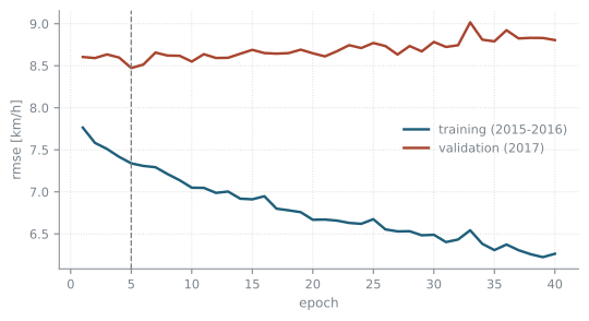
A network this large fits the training years better and better the longer it is trained, and the test years worse after a while. So we fit on 2015 and 2016, keep 2017 as a validation set, and stop at the epoch with the lowest validation error, as in early stopping. The test years 2019 and 2020 are used only once, at the end.
Code
import copyimport pandas as pdfrom sklearn.linear_model import LinearRegressionfrom sklearn.preprocessing import StandardScalerweather = pd.read_csv("https://go.epfl.ch/bio322-weather2015-2018.csv")weather_test = pd.read_csv("https://go.epfl.ch/bio322-weather2019-2020.csv")drop = ["LUZ_wind_peak", "time"]X = weather.iloc[:-5].drop(columns=drop).valuesy = weather["LUZ_wind_peak"].values[5:] # the wind peak five hours laterX_test = weather_test.iloc[:-5].drop(columns=drop).valuesy_test = weather_test["LUZ_wind_peak"].values[5:]year = weather["time"].values[:-5] //1_000_000fit, val = year <2017, year ==2017x_scaler = StandardScaler().fit(X[fit])y_scaler = StandardScaler().fit(y[fit].reshape(-1, 1))def to_tensor(A):return torch.tensor(x_scaler.transform(A), dtype=torch.float32)X_fit, X_val, X_te = to_tensor(X[fit]), to_tensor(X[val]), to_tensor(X_test)y_fit = torch.tensor(y_scaler.transform(y[fit].reshape(-1, 1)), dtype=torch.float32)def rmse(a, b):returnfloat(np.sqrt(np.mean((a - b) **2)))
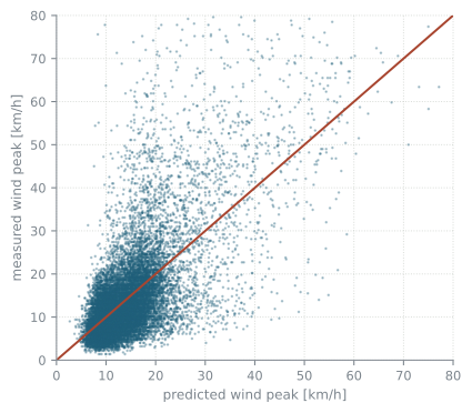
Figure 33.2: Predicted against measured wind peak on the test years 2019 and 2020. A perfect prediction would put every point on the diagonal.
If the model predicted the test data perfectly, all points would lie on the diagonal. They scatter widely around it, most likely because the irreducible error of this problem is large.
A network for the mean and the spread
A network can output more than a mean. With two outputs it can give the mean \(m(x)\) and the variance \(s(x)\) of a normal distribution for \(Y\,|\,x\), both non-linear functions of the input. The loss is the negative log-likelihood of the normal distribution, without its constant, \[
\mathcal L = \frac1n\sum_{i=1}^n \left(\frac{(y_i - m(x_i))^2}{2s(x_i)} + \frac12\log s(x_i)\right),
\] and the second output is passed through \(\mathrm{softplus}(z) = \log(1 + e^z)\), so that the variance is positive. We fit the logarithm of the wind peak five hours later against the pressure in Luzern, so that the fitted distribution of the wind peak itself is log-normal.
The first output is the mean, the second becomes the variance.
drawing the fitted mean and spread
grid = np.linspace(pressure.min(), pressure.max(), 200).reshape(-1, 1)with torch.no_grad(): out = net2(torch.tensor(px.transform(grid), dtype=torch.float32)).numpy()m = out[:, 0]sd = np.sqrt(np.log1p(np.exp(out[:, 1])))back =lambda z: np.exp(py.inverse_transform(z.reshape(-1, 1))[:, 0])fig, ax = plt.subplots(figsize=(8.8, 3.6))ax.plot(pressure[:, 0], np.exp(log_peak[:, 0]), "o", ms=4.5, mew=0.7, alpha=0.4, mfc="none", mec="#7a838b", rasterized=True) # open grey circles, for both themesax.plot(grid, back(m), color="#a8452f", lw=2.5, label="mean")ax.plot(grid, back(m + sd), color="#a8452f", lw=2, ls="--", label="± one standard deviation")ax.plot(grid, back(m - sd), color="#a8452f", lw=2, ls="--")ax.set(xlabel="LUZ_pressure [hPa]", ylabel="LUZ_wind_peak in 5 h [km/h]", ylim=(0, 115))ax.legend()plt.show()
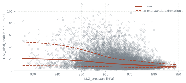
Figure 33.3: The wind peak five hours later against the pressure, with the fitted mean and one standard deviation on either side, all transformed back from the logarithm.
The mean depends slightly non-linearly on the pressure, and the spread of the wind peak is smaller at high pressure than at low pressure, where there are few points and several of them have high wind peaks. The dashed lines are not symmetric around the mean, because the fitted distribution is log-normal.