Tuning

Examples

Unless a section says otherwise, the panels and code blocks on this page use the data of resampling: points from \(f(x) = 0.3 + 2x - 0.8x^2 - 0.4x^3\) plus noise of standard deviation 1. The generator is a cubic, so the right answer for the polynomial degree is 3.

One hyper-parameter

Choosing the degree needs a score for every degree, and the split that chose it cannot also score it. Three arrangements, on the switch below.

• Validation set 10/10/80. 10% to fit each degree, 10% to score them, 80% held back. The best degree is refitted on the first 20% and scored on the 80%.
• 4-fold CV, all data. Every point is a validation point in one of the four folds. Nothing is left over to test with, so this setting tunes only.
• 4-fold CV on 20% + test set. The same cross-validation, on the same 20% the validation set approach used, with the other 80% kept as a test set — so the two are directly comparable.

Left, the validation loss at every degree for the current seed, its minimum, and where the strategy has a test set, the test error of the degree it chose. Right, the same curve for all 21 seeds at once, with each one’s minimum marked.

Two things to read off the right hand plot. Cross-validation finds the generator’s degree far more reliably: over the 21 seeds it picks degree 3 seventeen times out of twenty-one, against twelve for the validation set approach, which also wanders as far as degree 10.

And the score of the winner is not a test score. Averaged over the seeds, the validation set approach reports 1.06 for the degree it picked and that degree actually scores 1.45 on the held-out 80% — optimistic by 0.39. The cross-validated version on the same 20% reports 1.05 against a true 1.14. The gap is what you pay for using the same numbers to choose and to report.

GridSearchCV wraps a model, a list of values for a hyper-parameter and a resampling strategy into one estimator. Fitting it runs the cross-validation for every value and refits the best one on all the data.

import numpy as np
from sklearn.linear_model import LinearRegression
from sklearn.model_selection import GridSearchCV
from sklearn.pipeline import make_pipeline
from sklearn.preprocessing import PolynomialFeatures

def f(x):
    return 0.3 + 2 * x - 0.8 * x ** 2 - 0.4 * x ** 3

rng = np.random.default_rng(1)
x = rng.standard_normal(500)
y = f(x) + rng.standard_normal(500)
X = x.reshape(-1, 1)

model = make_pipeline(PolynomialFeatures(), LinearRegression())
search = GridSearchCV(model,
                      {"polynomialfeatures__degree": np.arange(1, 11)},
                      cv=10, scoring="neg_root_mean_squared_error")
search.fit(X, y)

print("best degree:", search.best_params_["polynomialfeatures__degree"])
print("its cross-validation RMSE:", round(-search.best_score_, 3))

1

The grid is keyed by <step name>__<parameter>. make_pipeline names a step after its class in lower case, so the degree of the PolynomialFeatures step is polynomialfeatures__degree. model.get_params() lists every name that can go on the left of that grid.

best degree: 3
its cross-validation RMSE: 1.063

Nothing in GridSearchCV is specific to polynomials. The number of neighbours of a kNN regression is tuned by the same call.

from sklearn.neighbors import KNeighborsRegressor

knn = GridSearchCV(KNeighborsRegressor(), {"n_neighbors": np.arange(1, 101)},
                   cv=10, scoring="neg_root_mean_squared_error")
knn.fit(X, y)

print("best k:", knn.best_params_["n_neighbors"])
print("its cross-validation RMSE:", round(-knn.best_score_, 3))

best k: 8
its cross-validation RMSE: 1.203

import matplotlib.pyplot as plt

ks = knn.cv_results_["param_n_neighbors"].astype(int)
fig, ax = plt.subplots(figsize=(8.8, 3.0))
ax.plot(ks, -knn.cv_results_["mean_test_score"])
ax.axvline(knn.best_params_["n_neighbors"], ls="--", lw=1, c="0.5")
ax.set(xlabel="k", ylabel="cross-validation RMSE")
plt.show()

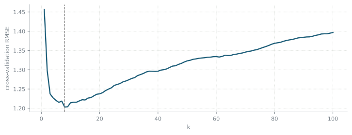
Figure 21.1: The 10-fold cross-validation RMSE of kNN regression on the 500 points, for every k from 1 to 100.

The curve runs the other way round from the degree: \(k = 1\) is the most flexible end, and the error falls from there to its minimum at \(k = 8\) before it climbs again. The best kNN, at 1.203, is still well behind the degree 3 polynomial, which has the generator’s own shape.

How reliable is the choice

The whole procedure repeated 200 times at each training set size. The dashed line is the true test error, measured on a large independent sample; the band is where the strategy’s estimate falls. The bars count how often each degree came out on top, with the true best degree picked out.

The band is widest for the single split at every \(n\), and it narrows as \(K\) grows. But look at the bars rather than the band: near the optimum the true error curve is almost flat, so a small amount of noise in the estimate moves the winning degree a long way, and more data does not rescue a single split.

Two hyper-parameters

Ridge regression on polynomial features has a degree and a penalty, and GridSearchCV crosses them. On the cubic data a penalty hardly matters, so this section uses the data of week 3: 50 points from \(f(x) = 0.3\sin(10x) + 0.7x\), with \(x\) uniform on \([0, 1]\) and noise of standard deviation 0.1.

from sklearn.linear_model import Ridge
from sklearn.preprocessing import StandardScaler

def f3(x):
    return 0.3 * np.sin(10 * x) + 0.7 * x

gen = np.random.default_rng(3)
x3 = gen.uniform(0, 1, 50)
X3, y3 = x3.reshape(-1, 1), f3(x3) + 0.1 * gen.standard_normal(50)

model2 = make_pipeline(PolynomialFeatures(), StandardScaler(), Ridge())
grid = GridSearchCV(model2,
                    {"polynomialfeatures__degree": np.arange(1, 21),
                     "ridge__alpha": np.logspace(-8, 2, 11)},
                    cv=5, scoring="neg_root_mean_squared_error")
grid.fit(X3, y3)

print("settings tried:", len(grid.cv_results_["params"]))
best = grid.best_params_
print("best degree:", best["polynomialfeatures__degree"],
      "  alpha:", best["ridge__alpha"])
print("its cross-validation RMSE:", round(-grid.best_score_, 3))

1

The same 50 training points as on the week 3 pages.

2

The penalty acts on the size of the coefficients, so the features are brought to one scale before it sees them.

settings tried: 220
best degree: 8   alpha: 0.0001
its cross-validation RMSE: 0.111

That is 220 settings and 1100 fits. The panel shows the same plane, with the number of settings as the budget.

The 5-fold cross-validation RMSE of every degree and penalty on the 50 points, darker where it is lower, and the settings a search strategy tries for a given budget. The triangle is the setting it returns.

The good settings form one valley: degrees from about 6 up, with a penalty between \(10^{-6}\) and \(10^{-3}\), and the higher the degree, the larger the penalty it needs. Too little penalty lets the high degrees overfit, too much makes every degree underfit. A grid only finds the valley if its points land in it. On the panel a 4 × 4 grid returns 0.112, next to the best on the plane, but a 5 × 5 grid only 0.121: the points move, and a larger grid is not always a better one.

Beyond the grid

RandomizedSearchCV draws the settings from distributions instead of a list. With the same budget it tries many more distinct values of each hyper-parameter, because no two settings share a row.

from scipy.stats import loguniform, randint
from sklearn.model_selection import RandomizedSearchCV

dist = {"polynomialfeatures__degree": randint(1, 21),
        "ridge__alpha": loguniform(1e-8, 1e2)}
rand = RandomizedSearchCV(model2, dist, n_iter=36, cv=5, random_state=0,
                          scoring="neg_root_mean_squared_error")
rand.fit(X3, y3)

best = rand.best_params_
print("best degree:", best["polynomialfeatures__degree"],
      "  alpha:", f"{best['ridge__alpha']:.2g}")
print("its cross-validation RMSE:", round(-rand.best_score_, 3))

1

randint(1, 21) draws the integers 1 to 20. loguniform is uniform in \(\log \alpha\), so each power of ten gets the same share of the draws.

best degree: 9   alpha: 0.00014
its cross-validation RMSE: 0.113

With 36 settings, a sixth of the grid, it comes within 0.002 of the full grid. On the panel, random search at 9 settings already covers nine degrees, against three for the 3 × 3 grid. Here the valley is wide, and from about 16 settings on both strategies land in it: random search is not better than a grid on this plane, only less sensitive to where the grid points happen to fall.

Successive halving spends the budget unevenly. It scores many candidates on a small part of the data, keeps the best third, triples the data, and repeats until the survivors are scored on all of it.

from sklearn.experimental import enable_halving_search_cv   # noqa: F401
from sklearn.model_selection import HalvingRandomSearchCV

halving = HalvingRandomSearchCV(model2, dist, cv=5, random_state=0,
                                scoring="neg_root_mean_squared_error")
halving.fit(X3, y3)

print("candidates per round:", halving.n_candidates_)
print("points per round:    ", halving.n_resources_)
best = halving.best_params_
print("best degree:", best["polynomialfeatures__degree"],
      "  alpha:", f"{best['ridge__alpha']:.2g}")
print("its cross-validation RMSE:", round(-halving.best_score_, 3))

1

The halving searches are still marked experimental, and this import is what switches them on.

2

Scored on the points of the last round, which with cv=5 is 30 of the 50: halving rounds the rounds to what the folds can split.

candidates per round: [5, 2]
points per round:     [10, 30]
best degree: 5   alpha: 9.4e-06
its cross-validation RMSE: 0.146

Here it does worst of all, on the panel at every budget too. Its first round ranks the candidates on a third of the data, where the scores are noisy and flexible settings look worse than they are, and it keeps the wrong ones. Halving is only as good as the ranking on a small part of the data.

Some models tune their own penalty. RidgeCV computes the leave-one-out error for every \(\alpha\) in its list from a single fit, so the search outside it only has to cover the degree.

from sklearn.linear_model import RidgeCV

model3 = make_pipeline(PolynomialFeatures(), StandardScaler(),
                       RidgeCV(alphas=np.logspace(-8, 2, 101)))
by_degree = GridSearchCV(model3, {"polynomialfeatures__degree": np.arange(1, 21)},
                         cv=5, scoring="neg_root_mean_squared_error")
by_degree.fit(X3, y3)

print("best degree:", by_degree.best_params_["polynomialfeatures__degree"])
print("its alpha:  ", f"{by_degree.best_estimator_[-1].alpha_:.2g}")
print("its cross-validation RMSE:", round(-by_degree.best_score_, 3))

best degree: 6
its alpha:   1e-08
its cross-validation RMSE: 0.115

Twenty settings on the outside and a hundred and one penalties on the inside, within 0.005 of the full 220-setting grid.

The score of the winner

Every search above reports the smallest of several noisy scores, and the smallest of several noisy numbers sits below the truth on average. This is the winner’s curse: the candidate that wins a noisy comparison has, on average, been lucky, so its score flatters it. The panel measures by how much. It draws 100 points from the same generator, tunes a kNN regression by 5-fold cross-validation, and compares the winner’s score with what the winner, refitted on all 100 points, does on 6000 new ones. It does this 250 times.¹

The switch picks what the candidates differ in.

	Values of k	A noise predictor
The model sees	\(x\)	\(x\) and one extra input that has nothing to do with \(y\)
The candidates differ in	the number of neighbours	which extra input it is
Number of neighbours	10 alone, then 9 to 11, 5 to 14, 1 to 30	always 10
In truth, the candidates are	nearly as good as each other	exactly as good as each other

250 repetitions on 100 points. The slider sets how many candidates the search compares. The dashed lines are the two means.

With one candidate there is nothing to choose and the score is a fair estimate. The search over \(k\) makes it optimistic, but only a little: with 30 values the winner’s score is 0.028 below its true error, and below it in 64% of the runs. Neighbouring values of \(k\) are scored on the same folds and give almost the same fit, so their scores rise and fall together and the smallest is barely below the rest.

The noise predictors have no such tie. Whichever one happens to line up with the noise in \(y\) on these folds wins, and new data does not share that noise. With 30 candidates the winner’s score is 0.086 below its true error, and below it in 86% of the runs. The more different the candidates, the more the search can find by chance.

The gap opens from both sides. The winner’s score falls as the search grows, but its true error also rises, from 1.059 to 1.070 over \(k\) and from 1.164 to 1.182 over the noise predictors. The more candidates there are, the more closely the choice follows the noise in this one sample: over 30 values of \(k\), one sample in eight picks a \(k\) below 5 or above 15, only because its noise made that \(k\) look best, and the runs that pick \(k\) below 5 do markedly worse on new data. The search itself overfits: every extra comparison is one more chance to fit the noise, and the variance this adds to the chosen model shows up as a higher test error.

Nested cross-validation

The fix is a second, outer split that the search never sees. For each of five outer folds the whole search runs again on the other four, and its winner is scored on the fold held out. The panel reports the mean of those five scores, for each of the same 250 samples.

The same 250 data sets, the same candidates and the same true test error as above, with the nested estimate in place of the winner’s own score.

For both searches and every number of candidates, the nested estimate lands within 0.016 of the true error on average and below it in fewer than half the runs. Its histogram is as wide as the winner’s — each estimate still rests on 100 held-out points — but it is no longer shifted.

Because every search object is itself an estimator, handing it to cross_val_score runs the search inside each outer fold.

from sklearn.model_selection import KFold, cross_val_score

outer = KFold(n_splits=5, shuffle=True, random_state=1)
nested = -cross_val_score(rand, X3, y3, cv=outer,
                          scoring="neg_root_mean_squared_error")

print("what the search reports:", round(-rand.best_score_, 3))
print("nested estimate:        ", round(nested.mean(), 3))

1

The inner cross-validation of rand chooses the degree and the penalty; the outer one scores the choosing. nested has one entry per outer fold, and each entry may come from a different setting — the nested estimate is of the procedure, not of any single model.

what the search reports: 0.113
nested estimate:         0.124

The search reports 0.113 for its winner; the procedure that produced it scores 0.124 on data it never saw. Report the nested number. Then fit the search once on all the data, as above, and ship the model it returns.

---

1. In both settings \(x \sim \mathcal U(-2, 2)\) and \(y = f(x) + \varepsilon\) with \(\varepsilon \sim \mathcal N(0, 1)\); \(x\) is uniform rather than normal so that no test point lies outside the range of the training data. Values of k: kNN on \(x\), with \(k\) in \(\{10\}\), \(\{9, 10, 11\}\), \(\{5, \dots, 14\}\) or \(\{1, \dots, 30\}\) for 1, 3, 10 or 30 candidates. A noise predictor: \(z_1, \dots, z_m \sim \mathcal U(-2, 2)\), with \(x, z_1, \dots, z_m\) and \(\varepsilon\) independent, so \(y\) does not depend on any \(z_j\); candidate \(j\) is kNN with \(k = 10\) on \((x, z_j)\), with the Euclidean distance. The true test error is the rmse of the refitted winner on 6000 new draws of \(x\), the \(z_j\) and \(y\).