Polynomial regression

Examples

Linear methods are not flexible enough

Two artificial data sets built from \(f(x) = 0.3\sin(10x) + 0.7x\): one for regression with a single predictor, one for binary classification.

import numpy as np
import pandas as pd

rng = np.random.default_rng(3)

def f(x):
    return 0.3 * np.sin(10 * x) + 0.7 * x

def logistic(z):
    return 1 / (1 + np.exp(-z))

def regression_data(n, sigma=0.1, rng=rng):
    x = rng.uniform(0, 1, n)
    return pd.DataFrame({"x": x, "y": f(x) + sigma * rng.standard_normal(n)})

def classification_data(n, s=20, rng=rng):
    X1, X2 = rng.uniform(0, 1, n), rng.uniform(0, 1, n)
    y = logistic(s * (f(X1) - X2)) > rng.uniform(0, 1, n)
    return pd.DataFrame({"X1": X1, "X2": X2, "y": y.astype(int)})

regression_train = regression_data(50)
classification_train = classification_data(400)

1

s is the steepness of the generator.

2

A point is labelled 1 with the probability the logistic function gives to \(s\,(f(X_1) - X_2)\), so the boundary between the two classes (at decision threshold 0.5) is the curve \(X_2 = f(X_1)\); a large s makes the labels near that curve less noisy.

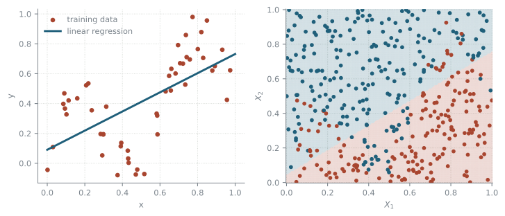
Figure 14.1: Left, linear regression on the regression data. Right, logistic regression on the classification data: the class it predicts at every point of a grid, with the training data on top.

There is structure in the training data that linear regression cannot capture, and the straight decision boundary cannot follow the curve the generator uses to separate the two classes.

Polynomial regression

One way to increase the flexibility is to fit a polynomial, which is linear regression on a transformed data set.

\[ \hat Y = \theta_0 + \theta_1 X + \theta_2 X^2 + \theta_3 X^3 + \cdots + \theta_d X^d \]

The transformation computes higher powers of the original input.

from sklearn.preprocessing import PolynomialFeatures

poly = PolynomialFeatures(degree=4, include_bias=False)
pd.DataFrame(poly.fit_transform(regression_train[["x"]]),
             columns=poly.get_feature_names_out()).head()

	x	x^2	x^3	x^4
0	0.085649	0.007336	0.000628	0.000054
1	0.236811	0.056079	0.013280	0.003145
2	0.801274	0.642041	0.514451	0.412216
3	0.582162	0.338913	0.197302	0.114862
4	0.094129	0.008860	0.000834	0.000079

Left, the training data, the fitted polynomial and the data generator. Right, the training and the test loss at every degree, the current degree marked on both curves, and the smallest test loss and the irreducible error as dashed lines. σ_gen is the noise level of the generator.

The training loss falls at every degree. The test loss does not: at \(\sigma_{\text{gen}} = 0.1\) it bottoms out around degree 8 at 0.109, never reaching the irreducible error of 0.1, and from degree 14 it climbs steeply and can be much worse than a straight line, depending on the noise level.

Fitting one is two steps in a pipeline: build the powers, then run least squares on them.

from sklearn.linear_model import LinearRegression
from sklearn.pipeline import make_pipeline

m = make_pipeline(PolynomialFeatures(degree=4, include_bias=False),
                  LinearRegression())
m.fit(regression_train[["x"]], regression_train["y"])
print("training MSE:",
      round(float(np.mean((m.predict(regression_train[["x"]])
                           - regression_train["y"]) ** 2)), 4))

1

A Pipeline refits the transformation whenever the model is refitted, which is what keeps the two in step.

training MSE: 0.0134

Polynomial classification

The same transformation applies to the classification data. Interestingly, even though the decision boundary (at a given decision threshold; 0.5 in the equation below) remains linear in the transformed features, i.e. for fixed parameters \(\theta_0, \ldots, \theta_{(d+1)(d+2)/2}\) the following equation describes a \((d+1)(d+2)/2\)-dimensional plane \[ \theta_0 + \theta_1X_1 + \theta_2X_2 + \theta_3X_1X_2 + \theta_4X_1^2 + \theta_5X_2^2 + \cdots + \theta_{(d+1)(d+2)/2}X_2^d = 0\, , \] it becomes an implicitly defined non-linear function in the \(X_1-X_2\) plane.

With two dimensional input the polynomial also contains mixtures like \(X_1X_2\) and \(X_1^2X_2\).

from sklearn.preprocessing import PolynomialFeatures

poly = PolynomialFeatures(degree=3, include_bias=False)
pd.DataFrame(poly.fit_transform(classification_train[["X1", "X2"]]),
             columns=poly.get_feature_names_out()).head()

	X1	X2	X1^2	X1 X2	X2^2	X1^3	X1^2 X2	X1 X2^2	X2^3
0	0.774105	0.389487	0.599238	0.301504	0.151700	0.463873	0.233395	0.117432	0.059085
1	0.393665	0.399647	0.154972	0.157327	0.159717	0.061007	0.061934	0.062875	0.063831
2	0.019600	0.705810	0.000384	0.013834	0.498167	0.000008	0.000271	0.009764	0.351611
3	0.527750	0.787720	0.278520	0.415719	0.620503	0.146989	0.219396	0.327470	0.488783
4	0.205232	0.115732	0.042120	0.023752	0.013394	0.008644	0.004875	0.002749	0.001550

Left, the class the fitted model predicts at every point of a grid, with the training data on top. Right, the negative log-likelihood against the degree. s_gen is the steepness of the logistic function in the generator.

The steeper the generator, the more flexibility pays: the best degree is 4 at \(s_{\text{gen}} = 5\) and 9 at \(s_{\text{gen}} = 30\). The irreducible error falls the same way, from 0.43 to 0.10, because a steep logistic function leaves less room for a label to come out either way.

from sklearn.linear_model import LogisticRegression

m = make_pipeline(PolynomialFeatures(degree=3, include_bias=False),
                  LogisticRegression(penalty=None, max_iter=2000))
m.fit(classification_train[["X1", "X2"]], classification_train["y"])
print("training accuracy:",
      round(m.score(classification_train[["X1", "X2"]],
                    classification_train["y"]), 3))

training accuracy: 0.873