More than two classes

Examples

The softmax

With \(C\) classes the model needs \(C\) probabilities that are positive and sum to one. We take one linear function per class, \(f_c(x) = \theta_{c0} + \theta_{c1}x_1 + \cdots + \theta_{cp}x_p\), and pass the vector of all \(C\) of them through the softmax, \[ P(Y = c\,|\,x) = s(f(x))_c = \frac{e^{f_c(x)}}{\sum_{k=1}^{C} e^{f_k(x)}} . \] The parameters form a \(C \times (p + 1)\) matrix \(\theta\). This model is called multinomial logistic regression, or linear classification. Its loss is again the negative log-likelihood, \(-\frac1n\sum_i \log P(Y = y_i\,|\,x_i)\), the cross-entropy.

Four classes and two inputs, so three parameters per class. Every point of the plane is coloured by the class with the largest probability, \(\arg\max_c s(f(x))_c\). The arrows are the weights \((\theta_{c1}, \theta_{c2})\) of each class, drawn twice as long. The sliders \(a_0\), \(a_1\), \(a_2\) add the same number \(a_0\) to every intercept and the same vector \((a_1, a_2)\) to every arrow. The black point is \(x = (1, 0)\).

Every boundary between two regions is a straight line, because every \(f_c\) is linear. The boundary between classes \(c\) and \(c'\) is where \(f_c = f_{c'}\), a line perpendicular to the difference of their arrows. Far from the origin the intercepts no longer matter, and in every direction the class whose arrow reaches furthest in that direction wins. Moving \(a_0\), \(a_1\) or \(a_2\) changes the arrows but neither the regions nor the probabilities at the black point: only the differences between the classes matter.

Fitting it by gradient descent

torch has cross_entropy, which takes the values \(f_c(x_i)\) and the integer labels, applies the softmax and returns the mean negative log-likelihood.

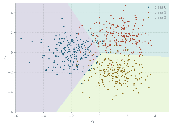
import numpy as np
import torch
import matplotlib.pyplot as plt

rng = np.random.default_rng(5)
C, p, n = 3, 2, 600
centers = np.array([[-2.0, 0.0], [1.5, 1.5], [1.0, -2.0]])
y = rng.integers(0, C, n)
X = centers[y] + rng.normal(0, 1.1, (n, p))            # three clouds of points
Xt = torch.tensor(X, dtype=torch.float64)
yt = torch.tensor(y, dtype=torch.long)

theta = torch.zeros((C, p + 1), dtype=torch.float64, requires_grad=True)

def f(theta, X):
    return theta[:, 0] + X @ theta[:, 1:].T

opt = torch.optim.Adam([theta], lr=0.05)
for step in range(400):
    opt.zero_grad()
    loss = torch.nn.functional.cross_entropy(f(theta, Xt), yt)
    loss.backward()
    opt.step()
print("cross-entropy after 400 steps:", round(float(loss), 4))

1

The \(C\) linear functions for every point at once, an \(n \times C\) matrix.

2

The mean negative log-likelihood of the labels.

cross-entropy after 400 steps: 0.2112

gx, gy = np.meshgrid(np.linspace(-6, 5, 220), np.linspace(-6, 5, 220))
G = torch.tensor(np.column_stack([gx.ravel(), gy.ravel()]))
with torch.no_grad():
    region = f(theta, G).argmax(dim=1).numpy().reshape(gx.shape)

fig, ax = plt.subplots()
ax.contourf(gx, gy, region, levels=[-.5, .5, 1.5, 2.5], alpha=0.18)
for c in range(C):
    ax.plot(X[y == c, 0], X[y == c, 1], ".", ms=4, label=f"class {c}")
ax.set(xlabel="$x_1$", ylabel="$x_2$")
ax.legend()
plt.show()

Figure 29.1: The data and the decision regions of the fitted model.

Linear classification of MNIST

The MNIST images have \(28 \times 28 = 784\) pixels and ten classes, so a linear classifier has ten linear functions of 784 inputs, \(10 \times 785 = 7850\) parameters. We fit it on the 60000 training images with Adam on batches of 128, and evaluate it on the 10000 test images.

from sklearn.datasets import fetch_openml

mnist = fetch_openml(data_id=554, as_frame=False, parser="auto")
X_all = (mnist.data / 255.0).astype(np.float32)          # pixels scaled to [0, 1]
y_all = mnist.target.astype(np.int64)
X_train, y_train = torch.tensor(X_all[:60000]), torch.tensor(y_all[:60000])
X_test, y_test = torch.tensor(X_all[60000:]), torch.tensor(y_all[60000:])

torch.manual_seed(1)
linear = torch.nn.Linear(784, 10)
opt = torch.optim.Adam(linear.parameters(), lr=1e-3)
loader = torch.utils.data.DataLoader(
    torch.utils.data.TensorDataset(X_train, y_train), batch_size=128, shuffle=True)

for epoch in range(10):
    for xb, yb in loader:
        opt.zero_grad()
        torch.nn.functional.cross_entropy(linear(xb), yb).backward()
        opt.step()

with torch.no_grad():
    train_acc = (linear(X_train).argmax(dim=1) == y_train).float().mean()
    test_acc = (linear(X_test).argmax(dim=1) == y_test).float().mean()
print(f"training accuracy {float(train_acc):.3f}, test accuracy {float(test_acc):.3f}")

1

torch.nn.Linear(784, 10) holds the \(10 \times 784\) weights and the ten intercepts, and computes all ten \(f_c(x)\) at once.

2

An epoch is one pass through all training images, here 469 batches.

training accuracy 0.929, test accuracy 0.926

Each class has one weight per pixel, so its 784 weights can be shown as an image.

w = linear.weight.detach().numpy()
fig, axes = plt.subplots(1, 10, figsize=(8.8, 1.2))
for c, ax in enumerate(axes):
    ax.imshow(w[c].reshape(28, 28), cmap="coolwarm", vmin=-np.abs(w).max(), vmax=np.abs(w).max())
    ax.set(xticks=[], yticks=[], title=str(c))
plt.show()

Figure 29.2: The weights of the ten linear functions, one image per digit. Red pixels raise the score of the digit, blue pixels lower it.

with torch.no_grad():
    pred = linear(X_test).argmax(dim=1).numpy()
wrong = np.where(pred != y_test.numpy())[0][:10]
fig, axes = plt.subplots(1, 10, figsize=(8.8, 1.3))
for ax, i in zip(axes, wrong):
    ax.imshow(X_test[i].reshape(28, 28), cmap="gray_r")
    ax.set(xticks=[], yticks=[], title=f"{int(y_test[i])} → {pred[i]}")
plt.show()

Figure 29.3: Test images the linear classifier gets wrong, with the true label and the prediction.