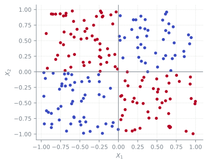
The XOR problem is a binary classification problem with two-dimensional input. The class is true if and only if the two coordinates of a point have different signs (exclusive or).
The decision boundary is not linear, and a linear logistic regression cannot separate the two classes.
linear = LogisticRegression(penalty=None).fit(X, y)print("training accuracy:", linear.score(X, y))
training accuracy: 0.69
Take the scalar product of the input with four different vectors, and set to 0 every scalar product that would be negative: \(H_j = \max(0, w_j^\top x)\) with \(w_1 = (1, 1)\), \(w_2 = (1, -1)\), \(w_3 = (-1, 1)\) and \(w_4 = (-1, -1)\). On these four features a linear logistic regression classifies every point correctly.
One column per vector: \(H_{ij} = \max(0, w_j^\top x_i)\).
training accuracy: 1.0
Learned vector features
Instead of choosing the four vectors, we can learn them with gradient descent, together with the coefficients of the logistic regression on top. The model has four hidden neurons \(\max(0, w_j^\top x)\) and a logistic output, \[
P(Y = \text{true}\,|\,x) = \sigma\Big(\beta_0 + \sum_{j=1}^{4}\beta_j\max(0, w_j^\top x)\Big),
\] 13 parameters in total, fitted by Adam on the negative log-likelihood.
Left, the data coloured by the prediction at step \(t\) at decision threshold 0.5, and the four vectors \(w_1, \dots, w_4\) as arrows. Right, the learning curve. The seed sets the starting point, \(0.1\) times a standard normal for every parameter.
The starting vectors depend on the seed, and so does the end: for 14 of the 20 seeds gradient descent finds a solution that classifies the training data (nearly) perfectly, for the other six it gets stuck at a training accuracy between 0.72 and 0.84.
More neurons than needed
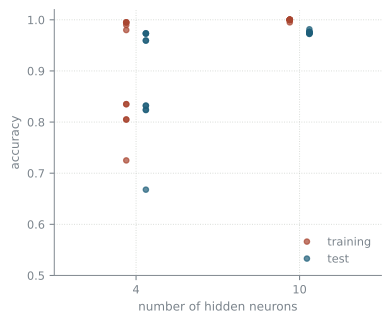
With more hidden neurons than the problem needs, gradient descent gets stuck less often. Below, a network with 4 and one with 10 hidden neurons are each fitted 10 times from different starting points, and evaluated on 10000 new points.
fitting 20 networks
import torchX_test =2* np.random.default_rng(2).random((10000, 2)) -1y_test = (X_test[:, 0] >0) != (X_test[:, 1] >0)Xt = torch.tensor(X, dtype=torch.float32)yt = torch.tensor(y, dtype=torch.float32)Xtt = torch.tensor(X_test, dtype=torch.float32)results = {}for m in [4, 10]: results[m] = []for run inrange(10): torch.manual_seed(run) net = torch.nn.Sequential(torch.nn.Linear(2, m), torch.nn.ReLU(), torch.nn.Linear(m, 1)) opt = torch.optim.Adam(net.parameters(), lr=1e-2)for step inrange(2000): opt.zero_grad() torch.nn.functional.binary_cross_entropy_with_logits( net(Xt)[:, 0], yt).backward() opt.step()with torch.no_grad(): train =float(((net(Xt)[:, 0] >0) == yt.bool()).float().mean()) test =float(((net(Xtt)[:, 0] >0).numpy() == y_test).mean()) results[m].append((train, test))fig, ax = plt.subplots(figsize=(4.4, 3.6))for k, m inenumerate([4, 10]): tr, te = np.array(results[m]).T ax.plot(np.full(10, k -0.06), tr, "o", color="C1", alpha=0.7, label="training"if k ==0elseNone) ax.plot(np.full(10, k +0.06), te, "o", color="C0", alpha=0.7, label="test"if k ==0elseNone)ax.set(xticks=[0, 1], xticklabels=["4", "10"], xlabel="number of hidden neurons", ylabel="accuracy", ylim=(0.5, 1.02), xlim=(-0.5, 1.5))ax.legend(loc="lower right")plt.show()
Figure 28.2: Training and test accuracy of 10 fits each of a network with 4 and with 10 hidden neurons.
With 4 neurons several fits get stuck in a solution that misclassifies a large part of the data. With 10 neurons none of them does, and all reach a test accuracy close to the best.