import numpy as np
import pandas as pd
import torch
import matplotlib.pyplot as plt
from sklearn.datasets import fetch_openml

mnist = fetch_openml(data_id=554, as_frame=False, parser="auto")
X_all = (mnist.data / 255.0).astype(np.float32)
y_all = mnist.target.astype(np.int64)
X_test, y_test = torch.tensor(X_all[60000:]), torch.tensor(y_all[60000:])
F = torch.nn.functionalRegularizing a network
Examples
Regularization helped the polynomials of week 3 and the logistic regression on spam. Can it also help a network?
Weight decay, dropout and early stopping
The L1 and L2 penalties are the same as for linear models,
\[ \mathcal L_{\text{reg}}(\theta) = \mathcal L(\theta) + \lambda\|\theta\|_2^2 \qquad\text{or}\qquad \mathcal L(\theta) + \lambda\|\theta\|_1 . \]
Two things are different. There is no closed form, so \(\lambda\) simply enters the gradient. And there is no unique optimum, so the penalty also decides which of many equally good solutions we end up in.
In deep learning the L2 penalty is usually called weight decay: its gradient \(2\lambda\theta\) pulls every parameter towards zero at every step.
Dropout sets a random fraction \(p\) of the activations to zero during training, and divides the rest by \(1-p\), so that the expected sum stays the same. At test time nothing is dropped. It forces the network not to rely on any single neuron. In torch it is nn.Dropout(p), and it is only active in training mode, so remember model.eval() before predicting.
Why should switching off neurons at random help? There are two ways to see it.
- No neuron can rely on another. A large network can fit noise by combining many neurons whose large contributions cancel each other almost exactly. Such a fit breaks as soon as one of them is missing. With dropout, every neuron has to be useful together with whichever random subset of the others happens to be there, so each random part of the network has to predict reasonably well on its own.
- An average of many networks. Every training step trains a different random subnetwork, and all of them share the same weights. The full network at test time behaves roughly like the average of all these subnetworks, and an average of many fits varies less than any one of them.
The panel shows both, on a network of 200 relu neurons fitted to 30 noisy points.
Without dropout the network passes close to every training point (training MSE 0.012, against a noise variance of 0.09) and its test error is lowest after about a hundred steps and rises from then on. Remove half of its neurons and its predictions leave the plot: the neurons only work together. Trained with dropout 0.5, every half network is a reasonable fit by itself, the full network is close to their average, and the test error keeps going down. The price is a training error at the level of the noise, which is where it should be.
Early stopping we already saw in week 5: stop the training when the validation loss stops improving.
MNIST with 1000 training images
With 60000 training images the network of week 6 hardly overfits. With 1000 it does: every model below classifies all its training images correctly.
def fit(X_train, y_train, weight_decay=0.0, dropout=0.0, epochs=200):
torch.manual_seed(1)
net = torch.nn.Sequential(
torch.nn.Linear(784, 100), torch.nn.ReLU(),
torch.nn.Dropout(dropout),
torch.nn.Linear(100, 10))
opt = torch.optim.Adam(net.parameters(), lr=1e-3,
weight_decay=weight_decay)
loader = torch.utils.data.DataLoader(
torch.utils.data.TensorDataset(X_train, y_train), batch_size=32, shuffle=True)
curve = []
for epoch in range(epochs):
net.train()
for xb, yb in loader:
opt.zero_grad()
F.cross_entropy(net(xb), yb).backward()
opt.step()
net.eval()
with torch.no_grad():
curve.append(-float(F.cross_entropy(net(X_test), y_test)))
with torch.no_grad():
accuracy = float((net(X_test).argmax(dim=1) == y_test).float().mean())
return accuracy, curve[-1], curve- 1
-
With
dropout=0.0this layer does nothing. - 2
-
weight_decayadds \(\lambda\theta\) to the gradient, which is the gradient of the penalty \(\frac{\lambda}{2}\|\theta\|_2^2\). - 3
-
Dropout is active in training mode only.
net.eval()switches it off for the evaluation after every epoch.
variants = {"no regularization": {},
            "weight decay 1e-3": {"weight_decay": 1e-3},
            "dropout 0.5": {"dropout": 0.5},
            "both": {"weight_decay": 1e-3, "dropout": 0.5}}
X_train, y_train = torch.tensor(X_all[:1000]), torch.tensor(y_all[:1000])
runs = {name: fit(X_train, y_train, **kw) for name, kw in variants.items()}
pd.DataFrame({name: {"test accuracy": a, "test log-likelihood": l}
for name, (a, l, _) in runs.items()}).T.round(3)| test accuracy | test log-likelihood | |
|---|---|---|
| no regularization | 0.878 | -0.743 |
| weight decay 1e-3 | 0.891 | -0.388 |
| dropout 0.5 | 0.886 | -0.667 |
| both | 0.891 | -0.401 |
fig, ax = plt.subplots(figsize=(6, 3.5))
for name, (_, _, curve) in runs.items():
    ax.plot(range(1, len(curve) + 1), curve, label=name)
ax.set(xlabel="epoch", ylabel="test log-likelihood per image")
ax.legend()
plt.show()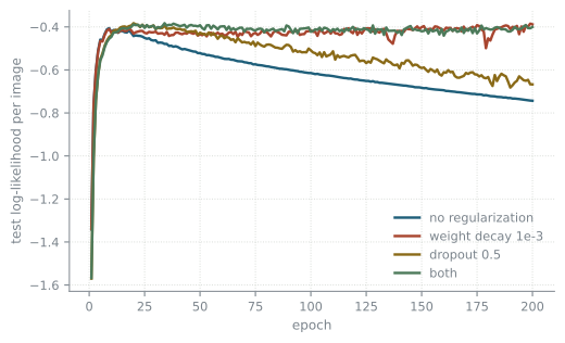
Regularization helps, a little in accuracy and a lot in log-likelihood, just as for the logistic regression on spam. Without it, the test log-likelihood is at its best after about 15 epochs and gets worse from then on, while the test accuracy hardly moves: the network keeps getting more confident, including about the images it gets wrong. Stopped at its best epoch, the unregularized network is about as good as the one with weight decay. That is why early stopping counts as a regularizer.
One run on one set of 1000 images could be luck. The same comparison on four other sets of 1000 training images:
rows = []
for k in range(1, 5):
    sl = slice(1000 * k, 1000 * (k + 1))
    X_k, y_k = torch.tensor(X_all[sl]), torch.tensor(y_all[sl])
    for name, kw in variants.items():
        accuracy, loglik, _ = fit(X_k, y_k, **kw)
        rows.append({"images": f"{1000 * k}-{1000 * (k + 1) - 1}", "model": name,
                     "test accuracy": accuracy, "test log-likelihood": loglik})
pd.DataFrame(rows).pivot(index="images", columns="model",
values=["test accuracy", "test log-likelihood"]).round(3)| test accuracy | test log-likelihood | |||||||
|---|---|---|---|---|---|---|---|---|
| model | both | dropout 0.5 | no regularization | weight decay 1e-3 | both | dropout 0.5 | no regularization | weight decay 1e-3 |
| images | ||||||||
| 1000-1999 | 0.892 | 0.889 | 0.877 | 0.888 | -0.410 | -0.673 | -0.747 | -0.411 |
| 2000-2999 | 0.889 | 0.892 | 0.885 | 0.893 | -0.420 | -0.659 | -0.726 | -0.397 |
| 3000-3999 | 0.882 | 0.875 | 0.874 | 0.883 | -0.443 | -0.747 | -0.747 | -0.415 |
| 4000-4999 | 0.892 | 0.893 | 0.884 | 0.891 | -0.413 | -0.642 | -0.748 | -0.410 |